
Return Back
Logo ARPM
Logo ARPM
contact us
start here
  • Bootcamp
    • Overview
    • Reviews
    • Info/FAQs
    • Enroll
  • Certification
    • Overview
    • Reviews
    • Info/FAQs
    • Enroll
  • Lab/Study materials
    • Overview
    • Machine Learning
    • Quant Finance
    • Primers
    • What's new
    • Enroll
  • start here login
contact us
login
Introduction
About the ARPM Lab
Learning the ARPM Lab by topic
Learning the ARPM Lab by channel
Audience and prerequisites
Notation
Key tenets
Indices
Special characters
Distributions
Portfolio
Glossary
Symbols
A
B
C
D
E
F
G
H
I
J
K
L
M
N
O
P
Q
R
S
T
U
V
W
Y
Z
Bibliography
Data science
[1]Summary: “Data Science Map”
[1.1]Probabilistic framework
[1.2]Mean-covariance framework
[1.3]Linear models
[1.4]Machine learning
[1.5]Estimation
[1.6]Inference
[1.7]Sequential decisions
I. Probabilistic framework
[2]Environment: probabilistic
[2.1]Distributions
[2.1.1]Cumulative distribution function
[2.1.2]Probability density function
[2.1.3]Probability mass function
[2.1.4]Characteristic function
[2.1.5]Additional representations
[2.2]Visualization
[2.3]Transformations
[2.3.1]Information set
[2.3.2]Marginalization
[2.3.3]Push-forward
[2.3.4]Law of the unconscious statistician
[2.3.5]Change of measure
[2.4]Functionals
[2.4.1]Key definitions
[2.4.2]Mode
[2.4.3]Quantile family
[3]Structure: conditional independence
[3.1]Independence
[3.2]Conditioning
[3.2.1]Conditional distribution
[3.2.2]Geometrical interpretation
[3.3]Bayes theorem
[3.3.1]Model
[3.3.2]Joint
[3.3.3]Compound
[3.3.4]Posterior
[3.4]Reduced-form representation
[3.4.1]Independent component analysis
[3.4.2]Multivariate quantile function
[3.4.3]Innovation extraction
[3.4.4]Stochastic functions
[3.5]Conditional independence
[3.6]Conditional functionals
[3.6.1]Mode
[3.6.2]Mean
[3.6.3]Variance
[3.6.4]ANOVA
[3.6.5]Quantile
[4]Jointness: copulas
[4.1]Grades and inverse sampling
[4.2]Definition of copula
[4.2.1]Absolutely continuous distribution
[4.2.2]General distribution
[4.2.3]Copula density function
[4.3]Properties of copulas
[4.3.1]Independence
[4.3.2]Comonotonicity
[4.3.3]Invariance
[4.4]Elliptical copulas
[4.4.1]Normal copula
[4.4.2]t copula
[4.4.3]Scenarios from elliptical copulas
[4.5]Archimedean copulas
[4.5.1]Scenarios from Archimedean copulas
[4.6]Implementation
[4.6.1]Copula-marginal separation
[4.6.2]Copula-marginal combination
[5]Distance: information geometry
[5.1]Distributions geometry
[5.1.1]Tangent vector
[5.1.2]Fisher metric: length and volume
[5.1.3]Flatness and geodesics
[5.1.4]Duality: potentials and Legendre transformations
[5.1.5]Distance and divergence
[5.2]Exponential distributions geometry
[5.3]Scenario-probability distribution geometry
[6]Stochastic optimization: decision theory
[6.1]Statistical decision problems
[6.1.1]State
[6.1.2]Action
[6.1.3]Loss function
[6.1.4]Reward
[6.2]Stochastic dominance
[6.2.1]Strong dominance
[6.2.2]Weak dominance
[6.2.3]Higher order dominance
[6.2.4]Stochastic dominance failure
[6.3]Bayes risk
[6.3.1]Problem without inputs
[6.3.2]Problem with inputs
[6.3.3]Bayesian approach
[6.3.4]Frequentist approach
[6.3.5]A unified view
[6.3.6]Admissibility
[6.4]Minimax and other approaches
[6.4.1]Minimax
[6.4.2]Minimax versus Bayes
[6.4.3]Generalizations
[6.5]Causality
[6.5.1]Observational decision problem
[6.5.2]Interventional decision problem
[6.5.3]From observations to interventions
[6.5.4]Selection of interventional variables
[6.6]Scoring rules
[6.6.1]Propriety
[6.6.2]Notable scoring rules
[6.6.3]Loss-implied scoring rules
[6.6.4]Beyond scoring rules
[6.7]Points of interest, pitfalls, practical tips
[6.7.1]Randomized decisions
[6.7.2]Improper priors
[6.7.3]Propriety
[6.7.4]Expected value of perfect and sample information
[7]Stochastic programming
[7.1]Definitions
[7.2]General tricks
[7.3]Functional fit
[7.3.1]Machine learning as functional optimization
[7.3.2]Parametric functional optimization
[7.4]Linear basis
[7.4.1]Interactions/polynomials
[7.4.2]Orthogonal series
[7.4.3]Error minimization
[7.5]Trees
[7.5.1]CART
[7.5.2]Splines
[7.5.3]Voronoi diagrams
[7.5.4]Error minimization
[7.6]Neural networks
[7.6.1]Neurons
[7.6.2]Neural networks
[7.6.3]Projection pursuit
[7.6.4]Error minimization
[7.7]Gradient boosting
[7.8]RKHS/Kernel trick
II. Mean-covariance framework
[8]Environment: mean-covariance
[8.1]Mean-covariance classes
[8.1.1]Mean vector
[8.1.2]Covariance matrix
[8.1.3]Equivalence class
[8.1.4]Z-score
[8.2]Visualization
[8.2.1]Spectral decomposition
[8.2.2]Mean-covariance ellipsoid
[8.2.3]Principal component analysis
[8.3]Affine transformations
[8.3.1]Mean vector
[8.3.2]Covariance matrix
[8.3.3]Linearized information set
[8.3.4]Marginalization
[8.3.5]Z-score invariance
[8.3.6]Higher order moments
[8.4]Elicitability
[8.4.1]Individual versus joint
[8.4.2]Minimum volume ellipsoid
[8.4.3]Minimum z-score parameters
[9]Structure: partial uncorrelation
[9.1]Uncorrelation
[9.2]Linear projection
[9.2.1]Predicted mean-covariance class
[9.2.2]Geometrical interpretation
[9.3]Linear Bayes theorem
[9.3.1]Model
[9.3.2]Joint
[9.3.3]Compound
[9.3.4]Posterior
[9.4]Reduced-form representation
[9.4.1]Uncorrelated component analysis
[9.4.2]Linear quantile function
[9.4.3]Linear innovation extraction
[9.4.4]Linear stochastic functions
[9.5]Partial uncorrelation
[9.6]Connections with conditional independence
[9.6.1]The normal case
[9.6.2]Linear approximation
[10]Jointness: correlation
[10.1]Mean-covariance grades
[10.2]Definition of correlation
[10.3]Properties of correlation
[10.3.1]Uncorrelation
[10.3.2]Affine concordance
[10.3.3]Invariance
[10.4]Related definitions
[11]Stochastic optimization: mean-variance trade-off
[11.1]Problem without inputs
[11.1.1]Mean-variance trade-off
[11.1.2]Solutions
[11.1.3]Alternative formulations
[11.1.4]Special cases
[11.2]Problem with inputs
[11.2.1]Posterior risk
[11.2.2]Joint risk
[11.2.3]Sparsity
[11.2.4]Weak signal
[11.2.5]A unified result
[11.3]Points of interest
[11.3.1]Affine actions
[12]Location and dispersion
[12.1]Affine equivariance
[12.1.1]Key definitions
[12.1.2]Mode/modal dispersion
[12.1.3]Median/interquantile range
[12.1.4]Multivariate extensions
[12.2]Variational principles
[12.2.1]Key definitions
[12.2.2]Elicitable and quadrangle features
[12.2.3]Quantile family
[12.2.4]Mean absolute deviation family
[12.2.5]Median absolute deviation
[12.2.6]Other locations/dispersions
[12.2.7]Multivariate extensions
[12.3]Points of interest, pitfalls, practical tips
[12.3.1]Visualization via uncertainty bands
[13]Dependence and concordance
[13.1]Measures of dependence
[13.1.1]Schweizer-Wolff measure
[13.1.2]Mutual information
[13.2]Measures of concordance
[13.2.1]Kendall’s tau
[13.2.2]Spearman’s rho
[13.3]Correlation as measure of dependence/concordance
[13.4]Points of interest, pitfalls, practical tips
[13.4.1]Schweizer and Wolff measure via simulations
III. Linear models
[14]Linear factor models
[14.1]Definitions
[14.1.1]The r-squared
[14.1.2]Dominant-residual models
[14.1.3]Systematic-idiosyncratic models
[14.1.4]Estimation
[14.2]Linear least squares regression models
[14.2.1]Definition
[14.2.2]Solution: factor loadings
[14.2.3]Prediction and fit
[14.2.4]Residuals features
[14.2.5]Natural scatter specification
[14.2.6]Estimation
[14.3]Principal component models
[14.3.1]Definition
[14.3.2]Solution: factor loadings and constructed factors
[14.3.3]Identification issues
[14.3.4]Prediction and fit
[14.3.5]Residuals features
[14.3.6]Natural scatter specification
[14.3.7]Estimation
[14.4]Factor analysis models
[14.4.1]Definition
[14.4.2]Solution: factor loadings and idiosyncratic variances
[14.4.3]Exact principal component with isotropic variances
[14.4.4]Identification issues
[14.4.5]Factor scores
[14.4.6]Prediction and fit
[14.4.7]Residuals features
[14.4.8]Natural scatter specification
[14.4.9]Estimation
[14.5]Cross-sectional models
[14.5.1]Definition
[14.5.2]Solution: factor-construction matrix
[14.5.3]Prediction and fit
[14.5.4]Residuals features
[14.5.5]Natural scatter specification
[14.5.6]Systematic-idiosyncratic assumption
[14.5.7]Estimation
[14.6]Points of interest, pitfalls, practical tips
[14.6.1]LFM’s are not a regression on past data(1) [⋆⋆]
[14.6.2]LFM’s are not about returns(2-3) [⋆⋆]
[14.6.3]LFM’s are not about stocks(4) [⋆⋆]
[14.6.4]LFM’s “factors”are not “factors returns”(5) [⋆]
[14.6.5]LFM’s are not systematic-idiosyncratic(6-7) [⋆⋆⋆]
[14.6.6]LFM’s are not horizon-independent(8) [⋆⋆]
[14.6.7]LFM’s are not a dimension reduction technique(9) [⋆]
[14.6.8]LFM’s are not APT and CAPM(10-11-12) [⋆⋆⋆]
[14.6.9]Factor analysis LFM’s are not idiosyncratic(14) [⋆⋆]
[14.6.10]LFM’s do not extract premia-generating factors(16)[⋆⋆]
[14.6.11]LFM’s are not always necessary(13-15-17-18) [⋆⋆⋆]
[14.6.12]Affine versus linear formulation
[14.6.13]Linear regression: a success story
[14.6.14]Principal factors are not principal components
[14.6.15]Performance of regression versus principal component
[14.6.16]Conditional principal component
[14.6.17]More general constraints
[15]Implicit dominant-residual models
[16]Structural equation models
IV. Machine learning
[17]Foundations
[17.1]Approaches to machine learning
[17.1.1]Supervised learning
[17.1.2]Unsupervised learning
[17.1.3]Reinforcement learning
[17.1.4]Linear factor models roots
[17.2]Prediction
[17.2.1]Point prediction
[17.2.2]Probabilistic prediction
[17.2.3]Point/probabilistic connections
[17.3]Learning and inference
[17.3.1]Learning
[17.3.2]Inference
[17.4]Points of interest, pitfalls, practical tips
[17.4.1]Marginalization and mode computation
[18]Supervised learning: regression
[18.1]Point least squares regression
[18.1.1]Error
[18.1.2]Theoretical optimum
[18.1.3]Optimization in practice
[18.1.4]Linear basis
[18.1.5]ANOVA
[18.1.6]Trees
[18.1.7]Neural networks
[18.1.8]Gradient boosting
[18.1.9]Kernel trick
[18.1.10]Geometrical interpretation
[18.2]Point non-least squares regression
[18.2.1]Error
[18.2.2]Theoretical optimum
[18.2.3]Optimization in practice
[18.2.4]Linear basis
[18.2.5]Advanced methods
[18.2.6]Generalized point regression
[18.3]Probabilistic regression
[18.3.1]Error
[18.3.2]Theoretical optimum
[18.3.3]Target parameters
[18.3.4]Optimization in practice
[18.3.5]Linear regression
[18.3.6]Generalized linear models
[18.3.7]Alternative generalizations
[18.4]Points of interest, pitfalls, practical tips
[18.4.1]Alternative errors
[18.4.2]Exponential tilting
[19]Supervised learning: classification
[19.1]Point binary classification
[19.1.1]Joint distribution
[19.1.2]Error
[19.1.3]Theoretical optimum
[19.1.4]Receiver operating characteristic (ROC)
[19.1.5]Optimization in practice
[19.1.6]Perceptron
[19.1.7]Support vector machines
[19.1.8]Fisher discriminant analysis
[19.2]Point multinomial classification
[19.2.1]Joint distribution
[19.2.2]Error
[19.2.3]Theoretical optimum
[19.2.4]Classification via discriminants
[19.2.5]Optimization in practice
[19.2.6]Leveraging binary classifiers
[19.3]Probabilistic classification
[19.3.1]Error
[19.3.2]Theoretical optimum
[19.3.3]Alternative approaches
[19.3.4]Target parameters
[19.3.5]Optimization in practice
[19.3.6]Logistic regression
[19.3.7]Naive Bayes classifiers
[19.3.8]Probit regression
[19.3.9]Neural networks
[19.3.10]Trees
[19.3.11]Gradient boosting
[19.4]Points of interest, pitfalls, practical tips
[19.4.1]Binary classification: alternative errors
[19.4.2]Linear regression for classification
[20]Unsupervised learning: autoencoders
[20.1]Least squares autoencoders
[20.1.1]Minimum torsion variables
[20.1.2]k-means clustering
[20.1.3]Kernel trick
[21]Unsupervised learning: graphical models
[21.1]Graphs
[21.2]Definitions
[21.3]Probabilistic factor analysis
[21.3.1]Solution: factor loadings and idiosyncratic variances
[21.3.2]Maximum likelihood factorization algorithm
[21.3.3]Special case: isotropic variances
[21.3.4]Identification issues
[21.3.5]Inference
[21.4]Mixture models
[21.4.1]Gaussian mixture models
[21.4.2]EM algorithm for Gaussian mixture models
[21.4.3]Inference
[21.4.4]Mixture of experts
[21.4.5]General mixtures models
[21.5]Naive Bayes models
[21.6]Bayes networks
[21.7]Markov networks
[22]Optimal transport
[22.1]General case
[22.1.1]Transport maps
[22.1.2]Monge problem
[22.1.3]Couplings
[22.1.4]Kantorovich problem
[22.1.5]Dual problem
[22.1.6]Wasserstein distance
[22.2]Categorical distributions
[22.2.1]Transport maps
[22.2.2]Monge problem
[22.2.3]Couplings
[22.2.4]Kantorovich problem
[22.2.5]Dual problem
[22.2.6]Wasserstein distance
[22.3]Histograms
[22.3.1]Transport maps
[22.3.2]Couplings
[22.3.3]Kantorovich problem
[22.3.4]Wasserstein distance
[22.4]Squared 2-norm loss
[22.4.1]Monge problem
[22.4.2]Kantorovich problem
[22.4.3]Dual problem
[22.4.4]Wasserstein distance
[22.4.5]Multivariate quantile function
[22.4.6]Polar decomposition
[22.4.7]Voronoi cells
[22.5]Linear optimal transport
[22.5.1]Linear transport maps
[22.5.2]Linear Monge problem
[22.5.3]Linear couplings
[22.5.4]Linear Kantorovich problem
[22.5.5]Dual Kantorovich problem
[22.5.6]Wasserstein distance
[22.5.7]Polar decomposition
[22.6]Earth mover problem
[22.6.1]General distance
[22.6.2]Histograms, q-norm
[22.6.3]Histograms, 0-1 distance
V. Estimation
[23]Estimation primer
[23.1]Flexible probabilities
[23.1.1]Exponential decay and time conditioning
[23.1.2]Kernels and state conditioning
[23.1.3]Joint state and time conditioning
[23.1.4]Statistical power of flexible probabilities
[23.2]Historical estimation
[23.2.1]Canonical historical estimation
[23.2.2]Generalization to flexible probabilities
[23.2.3]Extracting properties
[23.2.4]Exponential moving moments and statistics
[23.3]Kernel estimation
[23.3.1]Canonical kernel estimation
[23.3.2]Generalization to flexible probabilities
[23.4]Maximum likelihood estimation
[23.4.1]Maximum likelihood principle
[23.4.2]Canonical maximum likelihood for i.i.d. variables
[23.4.3]Generalization to flexible probabilities
[23.4.4]Extracting properties
[23.4.5]Exponential family (i.i.d.) assumption
[23.4.6]Generalization to non-i.i.d. observable processes
[23.5]Hidden variables and missing data
[23.5.1]Latent variables
[23.5.2]EM algorithm
[23.5.3]IID latent processes
[23.5.4]Markov state-space processes
[23.5.5]Networks
[23.5.6]Missing data
[23.6]Generalized method of moments
[23.6.1]Canonical method of moments
[23.6.2]Generalization to flexible probabilities
[23.6.3]Generalized method of moments - exact specification
[23.6.4]Generalized method of moments - over specification
[23.7]Robustness
[23.7.1]Local robustness
[23.7.2]Global robustness
[23.8]Bayesian estimation
[23.8.1]Estimation
[23.8.2]Prediction
[23.8.3]Analytical solutions
[23.8.4]Exponential family (i.i.d.) assumption
[23.9]Points of interest, pitfalls, practical tips
[23.9.1]Unconditional estimation
[23.9.2]Outlier detection
[23.9.3]Backward/forward exponential decay
[24]Estimation: location and dispersion
[24.1]Historical
[24.1.1]HFP mean, covariance and correlation
[24.1.2]HFP mean-covariance ellipsoid
[24.2]Maximum likelihood
[24.2.1]Normal assumption
[24.2.2]Student t assumption
[24.3]Missing data
[24.3.1]Randomly missing data
[24.3.2]Times series of different length
[24.4]Robustness
[24.4.1]High breakdown point with flexible probabilities estimators: theory
[24.4.2]High breakdown point with flexible probabilities estimators: practice
[24.5]Bayesian
[24.5.1]Model and sample estimators
[24.5.2]Normal-inverse-Wishart prior distribution
[24.5.3]Normal-inverse-Wishart posterior distribution
[24.5.4]Student t predictive distribution
[24.5.5]Classical equivalent, uncertainty and shrinkage
[24.6]Shrinkage
[24.6.1]Mean shrinkage: James-Stein
[24.6.2]Covariance shrinkage: Ledoit-Wolf
[24.6.3]Correlation shrinkage: random matrix theory
[24.6.4]Covariance shrinkage: sparse eigenvector rotations
[24.6.5]Covariance shrinkage: glasso
[24.6.6]Covariance shrinkage: factor analysis
[24.7]Mixed approach
[24.8]Frequentist risk: analytical results
[24.8.1]Sample mean/covariance
[25]Estimation: regression loadings
[25.1]Historical
[25.2]Maximum likelihood
[25.2.1]The model
[25.2.2]Normal assumption
[25.2.3]Student t assumption
[25.3]Bayesian
[25.3.1]The model
[25.3.2]Conditional likelihood and sample estimators
[25.3.3]Normal-inverse-Wishart prior distribution
[25.3.4]Normal-inverse-Wishart posterior distribution
[25.3.5]Student t predictive distribution
[25.3.6]Classical equivalent
[25.3.7]Uncertainty
[25.4]Regularization: factors selection
[25.4.1]Stepwise regression selection
[25.4.2]Lasso regression
[25.4.3]Ridge regression
[25.5]Mixed approach
[26]Random matrix theory
[26.1]Random matrix ensembles
[26.1.1]Eigenvalues
[26.1.2]Eigenvectors
[26.2]Empirical spectral distribution
[26.2.1]Probability density functions
[26.2.2]Cumulative distribution and quantile
[26.2.3]Moments
[26.2.4]Stieltjes transform
[26.2.5]Resolvent
[26.2.6]Replica
[26.2.7]Orthogonal transformations
[26.3]Infinite matrix limit
[26.3.1]Representations
[26.3.2]Deterministic convergence
[26.3.3]Stochastic convergence
[26.4]Boltzmann ensembles
[26.4.1]The ensembles
[26.4.2]Eigenvalues
[26.4.3]Eigenvectors
[26.4.4]Infinite matrix limit
[26.5]Wigner ensemble
[26.5.1]The ensemble
[26.5.2]Gaussian orthogonal ensemble
[26.5.3]Beyond Gaussian orthogonal
[26.6]Marchenko-Pastur ensemble
[26.6.1]The ensemble
[26.6.2]Addressing singularity
[26.6.3]Infinite matrix limit
[26.6.4]Wishart orthogonal ensemble
[26.6.5]Beyond Wishart orthogonal ensemble
[26.7]Free probability
[26.7.1]Scalars
[26.7.2]Matrices
[26.7.3]Infinite matrix limit
[26.7.4]Transforms
[26.7.5]Sums
[26.7.6]Products
[26.8]Dense covariances
[26.8.1]Samples with dense covariance
[26.8.2]Sample covariance revisited
[26.8.3]Limiting spectral density
[26.8.4]Application
[26.9]Spiked covariances
[26.9.1]Samples from linear factor models
[26.9.2]Sample covariance revisited
[26.9.3]Limiting spectral density
[26.9.4]Characteristic polynomial
[26.9.5]Free probability approach
[26.9.6]Outlier of the full covariance matrix
[27]Estimation theory: classical framework
[27.1]Definitions
[27.2]Bayesian
[27.3]Frequentist
[27.3.1]Risk
[27.3.2]Bias versus variance
[27.3.3]Minimax estimator
[27.4]Points of interest, pitfalls, practical tips
[27.4.1]Sample quantiles (order statistics)
[28]Hypothesis testing
[28.1]Single binary testing
[28.1.1]Tests
[28.1.2]P-value test
[28.2]Multiple binary testing
[28.3]Hypothesis testing for invariants
[28.3.1]Univariate testing: the z-statistic
[28.3.2]Multivariate testing: the Hotelling statistic
[29]Estimation theory: elicitable framework
[29.1]Definitions
[29.1.1]Predictive decision problem
[29.1.2]Estimative decision problem
[29.1.3]Sub-optimal two-step estimation
[29.1.4]New goal: oracle decision
[29.1.5]Optimal one-step estimation
[29.1.6]Conditional independence
[29.1.7]A unified view
[29.1.8]Conclusions
[29.2]Bayesian
[29.3]Frequentist
[29.3.1]Excess risk
[29.3.2]Empirical risk minimization
[29.3.3]Bias versus variance
[29.3.4]Approximation versus estimation
[29.3.5]Generalizations
[30]Estimation risk mitigation
[30.1]Bayesian
[30.2]Frequentist
[30.2.1]Ensemble
[30.2.2]Regularization
[30.2.3]Cross-validation
[30.2.4]Information criteria
[30.2.5]Best estimator
[30.3]Ensemble learning
[30.3.1]Bagging
[30.3.2]Flexible probabilities as random-variables
[30.3.3]Flexible probabilities through conditioning
[30.3.4]Ensemble weighting
[30.4]Regularization
[30.4.1]Stepwise features selection
[30.4.2]Ridge, lasso, elastic nets
[30.4.3]Glasso
[30.4.4]Categorical factors selection
[30.4.5]Bayesian prior
[30.4.6]Sparse principal component
[30.5]Cross-validation
[30.5.1]Background
[30.5.2]Estimation: in-sample error
[30.5.3]Testing: out-of-sample error
[30.5.4]Best estimator
[30.5.5]Cases of interest
[30.6]Information criteria and asymptotic theory
[30.7]Quest for invariance
[31]Invariance tests
[31.1]Simple tests
[31.2]Refinements and pitfalls
[31.2.1]Circle-like covariance (not data)
[31.2.2]Stronger tests based on copulas
VI. Inference
[32]Black-Litterman
[32.1]Prior distribution
[32.1.1]Performance model
[32.1.2]Prior distribution of expected returns
[32.1.3]Prior predictive performance distribution
[32.2]Active views
[32.2.1]Active views model
[32.2.2]Active views statement
[32.2.3]Posterior distribution of the expected returns
[32.2.4]Posterior predictive distribution
[32.3]Limit cases and generalizations
[32.3.1]High confidence in prior
[32.3.2]Low confidence in views
[32.3.3]High confidence in views
[32.3.4]Generalizations
[32.3.5]From linear returns to risk drivers
[32.3.6]From stock-like to generic asset classes
[32.3.7]From normal to non-normal markets
[32.3.8]From linear equality views to partial flexible views
[33]Generalized probabilistic inference
[33.1]Views processing: minimum relative entropy
[33.1.1]Base distribution and view variables
[33.1.2]Point views
[33.1.3]Distributional views
[33.1.4]Partial views
[33.1.5]Partial views on generalized expectations
[33.1.6]Sanity check
[33.1.7]Confidence
[33.1.8]Relationship with Bayesian updating
[33.2]Analytical implementation
[33.2.1]Base distribution
[33.2.2]Views
[33.2.3]Sanity check
[33.2.4]Updated distribution
[33.2.5]Confidence
[33.2.6]Relevant special cases
[33.3]Flexible probabilities implementation
[33.3.1]Base distribution
[33.3.2]Views
[33.3.3]Sanity check
[33.3.4]Updated distribution
[33.3.5]Confidence
[33.4]Factor-based implementations
[33.5]Copula opinion pooling
[33.5.1]Base distribution
[33.5.2]Views
[33.5.3]Updated distribution
[33.5.4]Confidence
[33.5.5]The algorithm
[33.6]Generalized shrinkage
[33.6.1]Intuition
[33.6.2]Classical shrinkage
[33.6.3]Bayesian updating
[33.6.4]Minimum relative entropy
[33.6.5]Shrinkage
[33.6.6]Regularization
[34]Inference via Monte Carlo and variational techniques
[34.1]Inference via Monte Carlo
[34.1.1]Metropolis-Hastings
[34.2]Inference and learning via variational techniques
[34.2.1]IM projection
[34.2.2]Inference
[34.2.3]Learning
[34.2.4]Analytical solution: exponential family
[34.2.5]Variational solution
[34.2.6]EM algorithm in population
[34.2.7]Dimension reduction
VII. Sequential decisions
[35]Stochastic processes environment
[35.1]Definitions
[35.1.1]Stochastic processes
[35.1.2]Paths
[35.1.3]Probabilistic specification
[35.1.4]Mean-covariance kernels
[35.2]Relevant properties
[35.2.1]Strong stationarity
[35.2.2]Covariance stationarity
[35.2.3]Ergodicity
[35.3]Prediction
[35.3.1]Probabilistic prediction
[35.3.2]Krieging
[35.3.3]Financial applications
[35.4]Points of interest
[35.4.1]Autocorrelation kernel
[35.4.2]Mean-covariance random fields
[35.4.3]Granger causality
[35.4.4]Linear decomposition
[35.4.5]Conditional expectation as best prediction
[35.4.6]General representation
[36]Random walk
[36.1]Strong white noise
[36.2]Discrete time random walk
[36.2.1]Definitions
[36.2.2]Relevant cases
[36.2.3]Forecast
[36.3]Levy processes
[36.3.1]Infinite divisibility
[36.3.2]Continuous state: Brownian diffusion
[36.3.3]Discrete state: Poisson jumps
[36.3.4]Notable Levy processes
[36.3.5]Levy-Khintchine representation
[36.3.6]Subordination
[36.3.7]Fourier algorithm for non- divisible processes
[36.4]Square-root rule and generalizations
[36.4.1]Thin-tailed random walk
[36.4.2]Thick-tailed random walk
[36.4.3]Multivariate random walk
[36.4.4]General processes
[36.5]Martingales
[37]Autoregressive processes
[37.1]Weak white noise
[37.1.1]Definition
[37.1.2]Relevant cases
[37.2]Autoregression of order one
[37.2.1]Definitions
[37.2.2]Stationarity
[37.2.3]Forecast
[37.3]Vector autoregression of order one
[37.3.1]Definitions
[37.3.2]Relevant cases
[37.3.3]Stationarity
[37.3.4]Cointegration
[37.3.5]Estimation
[37.3.6]Prediction
[37.4]Linear state-space models
[37.4.1]Definitions
[37.4.2]Relevant cases
[37.4.3]Stationarity
[37.4.4]Estimation
[37.4.5]Prediction - Kalman filter
[37.5]Ornstein-Uhlenbeck process
[37.5.1]Forecast and conditional distribution of OU
[37.5.2]Stationarity and unconditional distribution
[37.6]Multivariate Ornstein-Uhlenbeck
[37.6.1]Definitions
[37.6.2]Forecast and conditional distribution of MVOU
[37.6.3]Stationarity and unconditional distribution of MVOU
[37.6.4]Geometrical interpretation∗
[37.6.5]Cointegrated Ornstein-Uhlenbeck
[37.6.6]Relationship between (V)AR and (MV)OU
[37.7]Orthogonal increment processes
[38]Covariance stationary theory
[38.1]Spectral representation
[38.1.1]Spectral theorem - intuition
[38.1.2]Spectral theorem - formal statement
[38.1.3]Cramer decomposition - intuition
[38.1.4]Cramer decomposition - formal statement
[38.1.5]Application: identification
[38.2]Filtering
[38.2.1]Intuition
[38.2.2]Formal definitions
[38.2.3]autocovariance function
[38.2.4]Spectrum
[38.2.5]Affine equivariance
[38.2.6]Composition, inversion
[38.2.7]Causality
[38.2.8]Time domain filters
[38.2.9]Frequency domain filters
[38.3]Wold representation
[38.3.1]Intuition
[38.3.2]Formal statement
[38.3.3]Relationship with spectral analysis
[38.3.4]Computation of Wold components
[38.4]Dynamic factor models
[38.4.1]Dynamic regression
[38.4.2]Dynamic principal components
[39]Other mean-covariance stochastic models
[39.1](V)ARMA processes
[39.1.1]Definitions
[39.1.2]Stationarity
[39.1.3]Invertible (V)ARMA
[39.1.4]Forecast
[39.2]Integrated processes
[39.2.1]Integrated of order zero process
[39.2.2]Integer integration: ARIMA
[39.2.3]Fractional integration: fractional white noise
[39.3]Fractional Brownian motion
[39.4]Harmonic processes
[39.4.1]Definitions
[39.4.2]Relevant cases
[39.4.3]Mean and autocovariance
[39.4.4]Spectral density
[39.4.5]General basis as AR(2) limit
[39.4.6]Periodic harmonics as lagged AR(1) limit
[39.4.7]Multivariate harmonics
[39.4.8]Harmonics forecast
[39.5]Polynomial trend processes
[39.5.1]Definitions
[39.5.2]Stochastic approximations of deterministic trends
[39.5.3]Forecast
[40]Wiener-Kolmogorov filter
[40.1]From regression to filter
[40.2]Endogenous Wiener-Kolmogorov filter
[40.3]Exogenous Wiener-Kolmogorov filter
[41]Relevant probabilistic stochastic models
[41.1]Markov processes
[41.1.1]Theory
[41.1.2]Relevant cases
[41.2]Markov chains
[41.2.1]Time-homogeneous Markov chains
[41.2.2]Time-inhomogeneous Markov chains
[41.2.3]Multivariate Markov chain
[41.2.4]Continuous time-homogeneous Markov chain
[41.2.5]Continuous time-inhomogeneous Markov chains
[41.2.6]Stationarity and unconditional distributions
[41.3]State space processes
[41.3.1]Theory
[41.3.2]Probabilistic linear state-space models
[41.3.3]Hidden Markov models
[41.3.4]Hidden Markov VAR(1) models
[41.4]GARCH(1,1) process
[41.5]Stochastic volatility models
[41.5.1]State-space stochastic volatility
[41.5.2]Discrete time Heston model
[41.5.3]Hybrid models
[41.5.4]Continuous time Heston model
[41.5.5]Time changed Brownian motion
[41.5.6]Connection between time-changed Brownian motion and stochastic volatility
[41.6]Points of interest
[41.6.1]Probabilistic graphical models
[41.6.2]Markov property for random fields
[42]State-space forecasting
[42.1]Markov processes forecast
[42.1.1]Monte Carlo
[42.1.2]Historical bootstrapping
[42.1.3]Arbitrary monitoring times
[42.2]State-space processes forecast
[42.3]Points of interest
[42.3.1]Probabilistic forecast for general models
[42.3.2]Scenario projection enhancements by probability twisting
[42.3.3]Hybrid Monte Carlo-historical
VIII. Data science toolbox
[43]Linear algebra
[43.1]Vector spaces
[43.1.1]Vector operations
[43.1.2]Basis and coordinates
[43.1.3]Vector subspaces
[43.2]Linear transformations
[43.2.1]Matrix representation
[43.2.2]Composition
[43.2.3]Invertibility
[43.3]Inner product spaces
[43.3.1]Symmetry
[43.3.2]Positivity
[43.3.3]Length, distance and angle
[43.3.4]Orthogonal projection
[43.3.5]Best prediction
[43.3.6]Rotations
[43.4]Metric and normed spaces
[43.4.1]Norm
[43.4.2]Distance
[43.4.3]Divergence
[43.4.4]Geodesics
[43.5]Spectral decomposition
[43.5.1]Eigenvalues and eigenvectors
[43.5.2]Square matrix spectral decomposition
[43.5.3]Spectral theorem
[43.5.4]Singular value decomposition
[43.6]Matrix transpose-square-root
[43.6.1]Gramian
[43.6.2]Transpose-square-roots
[43.6.3]Orthonormalization
[43.6.4]Spectrum/principal components
[43.6.5]Cholesky/Gram-Schmidt
[43.6.6]Riccati/minimum torsion
[43.7]Matrix operations
[43.7.1]The vector space of matrices
[43.7.2]Key operations
[43.7.3]Pseudo-inverse
[43.7.4]Useful identities
[43.8]Matrix polynomials
[43.8.1]Matrix polynomials factorization
[43.8.2]Matrix polynomial inversion
[43.9]Pitfalls and points of interest
[43.9.1]Multiplicities
[44]Calculus
[44.1]Differentiation
[44.1.1]Univariate functions
[44.1.2]Multivariate functions
[44.1.3]Matrix-variate functions
[44.2]Taylor expansion
[44.2.1]Univariate functions
[44.2.2]Multivariate functions
[44.3]Integration
[44.3.1]Partitions and measurability
[44.3.2]Univariate integration
[44.3.3]Fundamental theorem of calculus
[44.3.4]Multivariate integration
[44.4]Monotone functions
[44.4.1]Univariate monotonicity
[44.4.2]Entrywise monotonicity
[44.4.3]Monotone maps
[44.5]Convexity
[44.5.1]Univariate convexity
[44.5.2]Multivariate convexity
[45]Optimization
[45.1]Fundamental concepts
[45.1.1]The optimization problem
[45.1.2]Local minimum
[45.2]Smooth programming
[45.2.1]First and second order criteria
[45.2.2]Lagrange multipliers
[45.2.3]Gradient descent
[45.2.4]Newton’s method
[45.3]Convex programming
[45.3.1]The general problem
[45.3.2]Linear programming
[45.3.3]Quadratic programming
[45.3.4]Second-order cone programming
[45.3.5]Semidefinite programming
[45.3.6]Conic programming
[45.4]Quadratic regularization
[45.4.1]Ridge regularization
[45.4.2]Lasso regularization
[45.4.3]Elastic net regularization
[45.5]Selection problems
[45.5.1]Problem statement
[45.5.2]General solution
[45.5.3]Combinatorial heuristics
[45.5.4]Elastic net heuristics
[45.6]Equivalent optimization problems
[45.6.1]Invertible function of the objective
[45.6.2]Epigraph form
[45.6.3]Slack variables
[46]Functional analysis
[46.1]Measure theory
[46.1.1]Domains
[46.1.2]Measures
[46.1.3]Lebesgue’s decomposition
[46.2]Functional algebra
[46.2.1]Function spaces
[46.2.2]Linear operators
[46.2.3]Kernel representation
[46.2.4]Eigenvalues and eigenfunctions
[46.3]L2 spaces
[46.3.1]Inner product
[46.3.2]Dirac delta
[46.3.3]Riesz representation theorem
[46.3.4]Unitary operators
[46.3.5]Lp geometry
[46.4]Fourier transform
[46.4.1]Intuition
[46.4.2]Toeplitz structure
[46.4.3]General transform and convolution
[46.4.4]Fourier integral transform
[46.4.5]Discrete time Fourier transform
[46.4.6]Fourier series
[46.4.7]Discrete Fourier transform
[46.5]Spectral theorem
[46.5.1]Motivation
[46.5.2]Mercer kernels
[46.5.3]Matrix-valued kernels
[46.6]Bochner’s theorem
[46.6.1]Spectral representation
[46.6.2]Power spectrum
[46.6.3]Matrix-valued kernels
[46.7]Mercer’s theorem
[46.7.1]Spectral representation
[46.7.2]Reproducing kernel Hilbert spaces
[46.7.3]Matrix-valued kernels
[46.8]Functional calculus
[46.8.1]Gateaux derivative
[46.8.2]Fréchet derivative
[46.8.3]Second order derivative
[47]Discrete mathematics
[47.1]Discrete derivatives
[47.1.1]Univariate derivatives
[47.1.2]Multivariate derivatives
[47.2]Combinatorial programming
[47.2.1]Brute force search
[47.2.2]Naive selection
[47.2.3]Stepwise forward selection
[47.2.4]Stepwise backward elimination
[47.2.5]2-step forward heuristic
[47.2.6]General combinatorial programming heuristics
[48]Abstract probability
[48.1]Key concepts
[48.1.1]Probability space
[48.1.2]Random variable
[48.1.3]Random fields
[48.1.4]Expectation
[48.1.5]Radon-Nikodym derivative
[48.1.6]Abstract distributions
[48.1.7]Conditional probability
[48.2]L2 spaces of random variables
[48.2.1]Inner product
[48.2.2]Length, distance and angle
[48.2.3]Visualization
[48.2.4]Geometry of random vectors
[48.2.5]Projection
[48.2.6]Covariance (improper) inner product
[48.3]Abstract conditional expectation
[48.3.1]Partitions of the sample space
[48.3.2]Probability conditional on a partition
[48.3.3]Discretization of random variables
[48.3.4]Conditional discretization of random variables
[48.3.5]Abstract Bayes theorem
[48.4]Abstract stochastic processes
[48.4.1]Filtrations
[48.4.2]Iterated expectations
[48.4.3]Adapted processes
[48.4.4]Martingales
[48.4.5]Approximations of processes
[49]Notable distributions
[49.1]Normal
[49.1.1]Pdf, cdf and characteristic function
[49.1.2]Moments
[49.1.3]Conditional distribution
[49.1.4]Stochastic representations
[49.1.5]Affine equivariance
[49.1.6]Matrix-normal
[49.1.7]Gaussian random fields
[49.2]Lognormal
[49.2.1]Pdf, cdf and characteristic function
[49.2.2]Moments
[49.2.3]Conditional distribution
[49.2.4]Shifted lognormal
[49.3]Quadratic normal
[49.3.1]Chi-squared
[49.3.2]Gamma
[49.3.3]Generalized chi-squared
[49.3.4]Wishart
[49.3.5]Inverse-Wishart
[49.4]Elliptical distributions
[49.4.1]Fundamental concepts
[49.4.2]Student t
[49.4.3]Cauchy
[49.4.4]Uniform inside the ellipsoid
[49.4.5]Uniform on the ellipsoid
[49.4.6]Affine equivariance
[49.4.7]Stochastic representations
[49.4.8]Generation of elliptical scenarios
[49.4.9]Scenario generation with dimension reduction
[49.5]Scenario-probability
[49.5.1]Types of scenario-probability distributions
[49.5.2]Probability mass and density function
[49.5.3]Transformations and generalized expectations
[49.5.4]Cumulative distribution function
[49.5.5]Quantile
[49.5.6]Moments and other statistical features
[49.6]Categorical
[49.6.1]Discriminant variables
[49.6.2]Probabilities parametrization
[49.7]Exponential family
[49.7.1]Normal
[49.7.2]Categorical
[49.8]Mixtures
[49.8.1]Binary case
[49.8.2]Multinomial case
[49.9]Stable, additive and infinitely divisible
[49.9.1]Stable
[49.9.2]Additive
[49.9.3]Infinitely divisible
[49.10]Moment-matching scenarios
[49.10.1]Twisting scenarios
[49.10.2]Twisting probabilities
Quantitative finance
[50]Summary: “Quantitative Finance Checklist”
[50.1]Financial engineering
[50.2]Risk management
[50.3]Portfolio management
[50.4]P versus Q
IX. Financial engineering
[51]Step 1: Valuation
[51a]Step 1a: Linear pricing theory - core
[51a.1]Fundamental axioms
[51a.1.1]Law of one price
[51a.1.2]Linearity
[51a.1.3]Absence of arbitrage
[51a.1.4]Relationships among fundamental axioms
[51a.2]Fundamental theorem of asset pricing
[51a.2.1]Linear pricing equation
[51a.2.2]Numeraire
[51a.2.3]Identification issues
[51a.3]Risk-neutral pricing
[51a.3.1]Discrete-time rebalancing
[51a.3.2]No rebalancing: forward measure
[51a.3.3]Continuous rebalancing limit
[51a.4]Capital asset pricing framework
[51a.4.1]Maximum Sharpe ratio portfolio
[51a.4.2]Security market line
[51a.4.3]Connections to CAPM and linear factor models
[51a.5]Covariance principle
[51a.5.1]Risk premium and equivalence with the security market line
[51a.5.2]Credit
[51a.5.3]Buhlmann exponential tilting
[51b]Step 1b: Linear pricing theory - further assumptions
[51b.1]Completeness
[51b.1.1]General statement
[51b.1.2]Arrow-Debreu securities
[51b.1.3]European options
[51b.2]Equilibrium: capital asset pricing model
[51b.3]Arbitrage pricing theory
[51b.3.1]Standard derivation: linear factor model for instruments
[51b.4]Intertemporal consistency
[51b.4.1]The framework
[51b.4.2]Intertemporal linear pricing equation
[51b.4.3]Intertemporal fundamental theorem of asset pricing
[51c]Step 1c: Non-linear pricing theory
[51c.1]Fundamental axioms
[51c.1.1]Law of one price
[51c.1.2]Non-linearity
[51c.1.3]Arbitrage
[51c.2]Valuation as evaluation
[51c.2.1]Variance and other shift principles
[51c.2.2]Certainty-equivalent principle
[51c.2.3]Distortion principles
[51c.2.4]Esscher principle
[51c.3]Intertemporal consistency
[51c.3.1]Continuous time variables
[51c.3.2]Non-linear “martingales”?
[51c.4]Point of interest and pitfalls
[51c.4.1]Linear (mis)uses of non-linear pricing
[51d]Step 1d: Valuation implementation
[51d.1]Equities
[51d.1.1]Discounted cash-flows
[51d.1.2]Multiples
[51d.2]Options
[51d.2.1]Bachelier
[51d.2.2]Black-Scholes
[51d.2.3]Heston
[51d.2.4]Valuation recipe
[51d.3]Fixed-income
[51d.3.1]Vasicek
[51d.3.2]Other models
[51d.3.3]Valuation recipe
[51d.4]Insurance
[51d.4.1]Life insurance
[51d.4.2]Non-life insurance
[51d.5]Real assets
[52]Step 2: Risk drivers identification
[52.1]Equities
[52.2]Fixed-income
[52.2.1]Rolling value
[52.2.2]Yield to maturity
[52.2.3]Alternative representations
[52.2.4]Parsimonious representations
[52.2.5]Spreads
[52.3]Derivatives
[52.3.1]Rolling value
[52.3.2]Implied volatility
[52.3.3]Alternative representations
[52.3.4]Parsimonious representations
[52.3.5]Risk drivers for a variance swap
[52.4]Commodities
[52.5]Credit
[52.5.1]Modelling default
[52.5.2]Ratings as risk drivers
[52.5.3]Risk drivers from conditioning
[52.6]Currencies
[52.7]Insurance
[52.8]Operations
[52.9]High frequency
[52.10]Strategies
[52.11]Points of interest, pitfalls, practical tips
[52.11.1]Spurious heteroscedasticity
[53]Step 3: Quest for invariance
[53a]Step 3a: Univariate quest for invariance
[53a.1]Efficiency
[53a.1.1]Heavy tails increments
[53a.1.2]Skewed and positive distributions
[53a.1.3]Stochastic volatility increments
[53a.1.4]Discrete increments
[53a.2]Trends
[53a.2.1]Deterministic trend
[53a.2.2]Stochastic trend
[53a.3]Seasonality
[53a.4]Short memory
[53a.5]Long memory
[53a.6]Volatility clustering
[53a.6.1]Price clustering
[53a.6.2]Time clustering
[53a.7]Discrete migrations
[53a.7.1]Markov chains
[53a.7.2]Structural models
[53a.8]Points of interest
[53a.8.1]Returns are not invariants
[53a.8.2]Sampling step size
[53b]Step 3b: Multivariate quest and forecasting
[53b.1]Mean-covariance approach
[53b.1.1]Mean reversion
[53b.1.2]Cointegration
[53b.1.3]Mean-covariance/analytical forecast
[53b.2]Probabilistic historical approach
[53b.2.1]Historical distribution
[53b.2.2]Historical forecast
[53b.3]Probabilistic copula-marginal approach
[53b.3.1]Static copula-marginal
[53b.3.2]Credit application
[53b.3.3]Dynamic copula-marginal
[53b.3.4]Copula-marginal forecast
[54b.4]Points of interest
[54b.4.1]Probabilistic, multivariate quest for invariance
[54b.4.2]Toward machine learning
[54b.4.3]Dynamic copula marginal forecast
[54b.4.4]Standardization
[54b.4.5]Non-synchronous data
[54b.4.6]Historical forecast with consecutive (non-)overlapping sequences
[54b.4.7]High-frequency volatility/correlation
[55]Step 4: Repricing
[55.1]Repricing functions
[55.1.1]Full repricing
[55.1.2]Carry
[55.1.3]Taylor approximation
[55.2]Techniques
[55.2.1]Scenario-based full repricing
[55.2.2]Analytical Taylor repricing
[55.2.3]Hybrid Taylor/full repricing
[55.2.4]Testing the repricing
[55.3]Equities
[55.3.1]Full repricing
[55.3.2]Carry
[55.3.3]Taylor approximation
[55.4]Fixed-income
[55.4.1]Zero-coupon bonds
[55.4.2]Coupon bonds
[55.4.3]Carry
[55.4.4]Taylor approximation
[55.5]Derivatives
[55.5.1]European call options
[55.5.2]Taylor approximation
[55.5.3]Variance swap
[55.5.4]Carry
[55.5.5]Taylor approximation
[55.6]Credit
[55.6.1]Full repricing
[55.6.2]Simplified regulatory framework
[55.7]Currencies
[55.7.1]Exchange rates
[55.7.2]Forward contracts
[55.7.3]Carry
[55.8]Pitfalls and practical tips
[55.8.1]Strategies
[55.8.2]Repricing and arbitrage
[55.8.3]Path dependence
[55.8.4]“Repricing”versus “asset pricing/valuation theory”
[55.8.5]Black-Scholes-Merton is exactly correct!
[55.8.6]Greeks for intra-day updates
[55.8.7]Greeks at the horizon
[55.8.8]Bond carry versus accrued interest
[55.8.9]Option carry versus theta
X. Risk management
[56]Step 5: Aggregation
[56a]Step 5a: Value aggregation
[56a.1]Portfolio value
[56a.1.1]Linear portfolio value
[56a.1.2]Sum-of-parts
[56a.1.3]Valuation recipe
[56a.1.4]Portfolio exposure
[56a.2]Portfolio weights
[56a.2.1]Generalized weights
[56a.2.2]Offset cash
[56a.3]Credit value adjustment
[56a.3.1]Counterparty credit risk exposure
[56a.3.2]Credit value adjustment computation
[56a.4]Liquidity value adjustment
[56a.5]Points of interest and pitfalls
[56a.5.1]Horizon-dependent exposure
[56a.5.2]Diffusive exposure
[56a.5.3]Solvency and collateral
[56b]Step 5b: Performance aggregation
[56b.1]Static market/credit risk
[56b.1.1]P&L
[56b.1.2]Returns
[56b.1.3]Benchmark
[56b.1.4]Scenario-probability distribution
[56b.1.5]Elliptical distribution
[56b.1.6]Quadratic-normal distribution
[56b.2]Dynamic market/credit risk
[56b.2.1]Portfolio rebalancing P&L
[56b.2.2]Allocation policy P&L
[56b.3]Stress-testing
[56b.3.1]Theory
[56b.3.2]Why have stress-tests
[56b.3.3]Panic copula
[56b.3.4]Extreme copula
[57]Step 6: Ex-ante evaluation
[57.1]Stochastic dominance
[57.2]Satisfaction/risk measures
[57.3]Mean-variance trade-off
[57.3.1]Mean
[57.3.2]Variance
[57.3.3]Standard deviation
[57.3.4]Mean-variance trade-off
[57.3.5]A strange success story
[57.4]The fundamental risk quadrangle
[57.4.1]Relevant cases
[57.4.2]Generalizations
[57.5]Expected utility and certainty-equivalent
[57.5.1]Common examples
[57.5.2]Computation
[57.6]Value at Risk and quantile
[57.6.1]Definition
[57.6.2]Computation
[57.7]Expected shortfall and sub-quantile
[57.7.1]Definition
[57.7.2]Computation
[57.8]Spectral/distortion satisfaction measures
[57.8.1]Definition
[57.8.2]Common examples
[57.8.3]Computation
[57.9]Coherent satisfaction measures
[57.9.1]Definition
[57.9.2]Common examples
[57.9.3]Computation
[57.10]Induced expectations
[57.10.1]Definition
[57.10.2]Common examples
[57.10.3]Computation
[57.11]Non-dimensional ratios
[57.11.1]Signal-to-noise ratio
[57.11.2]Downside ratios
[57.11.3]Correlation
[57.12]Pitfalls, points of interest and practical tips
[57.12.1]The Arrow-Pratt approximation of the certainty-equivalent
[57.12.2]Utility versus quantile
[57.12.3]Utility versus spectrum functions
[57.12.4]The Buhlmann and Esscher expectations are not distortion expectations
[57.12.5]Satisfaction measures under normality
[58]Step 7: Ex-ante attribution
[58a]Step 7a: Ex-ante performance attribution
[58a.1]Bottom-up exposures
[58a.1.1]Pricing factors
[58a.1.2]Style factors/smart beta
[58a.2]Top-down exposures: factors on demand
[58a.2.1]Analytical computation
[58a.2.2]Cardinality constraints
[58a.3]Relationship between bottom-up and top-down exposures
[58a.3.1]Subportfolios
[58a.4]Joint distribution
[58a.4.1]Elliptical distribution
[58a.4.2]Scenario-probability distribution
[58a.5]Application: hedging
[58a.6]Pitfalls and practical tips
[58a.6.1]Estimation versus attribution
[58a.6.2]The ex-ante attribution is not a regression on past data
[58b]Step 7b: Ex-ante risk attribution
[58b.1]General criteria
[58b.1.1]Isolated/“first in”proportional attribution
[58b.1.2]“Last in”proportional attribution
[58b.1.3]Sequential attribution
[58b.1.4]Shapley attribution
[58b.2]Euler decomposition
[58b.2.1]Standard deviation and variance
[58b.2.2]Certainty-equivalent
[58b.2.3]Quantile
[58b.2.4]Sub-quantile
[58b.2.5]Spectral satisfaction measures
[58b.2.6]Coherent measures
[58b.3]Linear attribution for induced expectations
[58b.3.1]Actuarial pricing
[58b.4]Minimum-torsion bets attribution of variance
[58b.4.1]Minimum-torsion bets
[58b.4.2]Effective number of bets
[59]Enterprise risk management
[59.1]General approach
[59.1.1]Portfolio: balance sheet
[59.1.2]Performance: income statement
[59.2]Banking regulatory framework
[59.2.1]Economic net income
[59.2.2]Default events
[59.2.3]Conditional losses
[59.2.4]Vasicek model
[59.2.5]Economic capital
[59.2.6]Risk attribution
[59.3]Insurance regulatory framework
[59.3.1]Economic net income
[59.3.2]Solvency capital requirement
[59.4]Points of interest
[59.4.1]CreditRisk+ approximation
XI. Portfolio management
[60]Step 8: Construction
[60a]Step 8a: Portfolio optimization
[60a.1]Mean-variance framework
[60a.1.1]Special portfolios
[60a.1.2]Quadratic target formulation
[60a.1.3]Linear target formulation
[60a.1.4]Setting the inputs
[60a.2]Analytical mean-variance
[60a.2.1]Total return
[60a.2.2]Excess return over risk-free
[60a.2.3]Excess return over benchmark
[60a.2.4]Total versus excess return
[60a.3]Numerical mean-variance
[60a.3.1]Constraints on positions/trade size
[60a.3.2]Constraints on number of positions
[60a.3.3]Transaction costs
[60a.4]Fundamental law of active management
[60a.4.1]Monetary impact of one signal
[60a.4.2]Information coefficient
[60a.4.3]Monetary impact of multiple signals
[60a.4.4]Aggregation
[60a.4.5]Transfer coefficient
[60a.5]Pitfalls, points of interest and practical tips
[60a.5.1]Black-Litterman equilibrium inputs via minimum relative entropy
[60b]Step 8b: Estimation and model risk
[60b.1]Mean-variance estimation risk measurement
[60b.1.1]Allocation as estimation
[60b.1.2]From predictive to estimative decisions
[60b.1.3]Two extreme allocation decisions
[60b.1.4]Decision theoretic allocation loss
[60b.2]Mean-variance Bayesian optimization
[60b.3]Mean-variance frequentist optimization
[60b.3.1]Tractable hypothesis set
[60b.3.2]Robust frontier
[60b.4]Probabilistic estimation risk measurement
[60b.4.1]Allocation as estimation
[60b.4.2]From predictive to estimative decisions
[60b.4.3]Probabilistic Bayesian optimization
[60b.4.4]Probabilistic frequentist optimization
[60b.4.5]Two-step approach
[60c]Step 8c: Cross-sectional strategies
[60c.1]Signals
[60c.1.1]Carry signals
[60c.1.2]Value signals
[60c.1.3]Technical signals
[60c.1.4]Fundamental and other signals
[60c.1.5]Signal processing
[60c.2]Premia
[60c.2.1]Signal-induced factor
[60c.2.2]Backtesting
[60c.3]Direct construction from signals
[60c.3.1]Signals as decision rules
[60c.4]Construction from signal predictions
[60c.4.1]Characteristic portfolio
[60c.4.2]Flexible factor
[60c.5]Relationship to APT
[60c.6]Multiple signals
[60c.6.1]Factor-mimicking portfolios
[60c.6.2]Relationship to APT
[60c.7]Points of interest, pitfalls, practical tips
[60c.7.1]Machine learning
[60d]Step 8d: Time series strategies
[60d.1]The market
[60d.1.1]Risky investment
[60d.1.2]Low-risk investment
[60d.1.3]Strategies
[60d.2]Expected utility maximization
[60d.2.1]The objective
[60d.2.2]Optimization
[60d.3]Option based portfolio insurance
[60d.3.1]Payoff design
[60d.3.2]Partial differential equation
[60d.3.3]Budget
[60d.3.4]Policy
[60d.3.5]A unified approach
[60d.4]Rolling horizon heuristics
[60d.4.1]Constant proportion portfolio insurance
[60d.4.2]Drawdown control
[60d.5]Signal induced strategy
[60d.6]Convexity analysis
[61]Step 9: Execution
[61.1]Market impact modeling
[61.1.1]Exogenous impact
[61.1.2]Endogenous impact
[61.2]Order scheduling
[61.2.1]Trading P&L decomposition
[61.2.2]Model P&L
[61.2.3]Moments of model P&L
[61.2.4]Model P&L optimization
[61.2.5]Quasi-optimal P&L distribution
[61.3]Order placement
[61.3.1]Step 1: Order scheduling
[61.3.2]Step 2: Order placement
[61.4]Microstructure signals
[61.4.1]Trade autocorrelation
[61.4.2]Order imbalance
[61.4.3]Price prediction
[61.4.4]Volume clustering
[61.5]Points of interest, pitfalls, practical tips
[61.5.1]Mean-variance optimization in complex models
[61.5.2]Price manipulation
[61.5.3]Testing
[62]Step 10: Ex-post performance analysis
XII. Finance toolbox
[63]Foundations
[63.1]Instrument value
[63.1.1]Fair value
[63.1.2]Transaction value
[63.1.3]Value versus price
[63.1.4]Exposure
[63.1.5]Leverage
[63.2]Portfolio value
[63.2.1]Long positions
[63.2.2]Short positions
[63.2.3]Generic positions
[63.3]Cashflows
[63.3.1]The jump rule
[63.3.2]Cumulative cashflows
[63.3.3]Re-invested cash-flows
[63.3.4]Cashflow adjusted value
[63.4]Market microstructure
[63.4.1]Limit order book
[63.4.2]Co-moving values
[63.4.3]Transaction variables
[63.4.4]Activity time
[63.4.5]Liquidity curve
[64]Performance definitions
[64.1]Profit-and-loss and payoff
[64.1.1]Profit-and-loss (P&L)
[64.1.2]Payoff
[64.2]Holding P&L of a position
[64.2.1]Long positions
[64.2.2]Short positions
[64.2.3]Generic positions
[64.3]Trading P&L of a position
[64.3.1]Single transaction
[64.3.2]Multiple transactions in one position
[64.4]Implementation shortfall
[64.5]Returns
[64.5.1]Basic definitions
[64.5.2]Generalized linear returns
[64.5.3]Excess returns
[64.5.4]Investments with capital injection
[64.5.5]Log-returns
[64.6]Path analysis
[64.7]Pitfalls and practical tips
[64.7.1]Linear versus compounded returns
[64.7.2]Multi-currency conversions
[64.7.3]Actual versus simple P&L
[65]Asset classes
[65.1]Equities
[65.2]Fixed-income
[65.2.1]Zero-coupon bond
[65.2.2]Bank account
[65.2.3]Coupon bond
[65.2.4]Interest rate swaps
[65.2.5]Amortizing financial instruments
[65.3]Derivatives
[65.3.1]Call/put option
[65.3.2]Futures
[65.3.3]Variance swaps
[65.4]Commodities
[65.5]Credit
[65.5.1]Default variables
[65.5.2]P&L in the presence of credit risk
[65.5.3]Spreads
[65.6]Foreign exchange
[65.6.1]Forward exchange rate
[65.6.2]Forward contracts
Case studies
XIII. Quantitative finance: the “Checklist”
[66]Monte Carlo Checklist
[66.1]Step 2: Risk drivers identification
[66.1.1]Market
[66.1.2]Credit
[66.2]Step 3: Quest for invariance
[66.2.1]Market
[66.2.2]Credit
[66.3]Step 4: Repricing
[66.4]Step 5: Aggregation
[66.5]Step 6: Ex-ante evaluation
[66.6]Step 7: Ex-ante attribution
[66.6.1]Ex-ante attribution: performance
[66.6.2]Ex-ante attribution: risk
[66.7]Step 8: Construction
[66.8]Step 9: Execution
XIV. Data science: factor models and learning
[67]Principal component analysis of the yield curve
[67.1]Cross-sectional structure of the yield curve covariance
[67.2]Finite set of times to maturity
[67.3]The continuum limit
[68]Machine learning for hedging
[68.1]Least squares regression
[68.1.1]Theoretical optimum
[68.1.2]Linear least squares regression
[68.1.3]Least squares regression tree
[68.2]Least absolute distance regression
[68.2.1]Theoretical optimum
[68.2.2]Linear least absolute distance regression
[68.2.3]Least absolute distance regression tree
[69]Machine learning for credit risk
[69.1]Credit default classification
[69.1.1]Background
[69.1.2]Fit and assessment
[69.1.3]Logistic regression
[69.1.4]Interactions
[69.1.5]Encoding
[69.1.6]Regularization
[69.1.7]Trees
[69.1.8]Gradient boosting
[69.1.9]Cross-validation
[70]Clustering for the stock market
[70.1]k-means clustering
[70.2]Shrinkage

24.5 Bayesian PIC

Key points

  • The normal-inverse-Wishart model is a tractable model for the Bayesian estimation of location and dispersion of a strong white noise.
  • The estimation model is normal (24.39); the prior distribution of the parameters is normal-inverse-Wishart (24.45)-(24.46); the posterior distribution is also normal-inverse-Wishart (24.53)-(24.54), with updated parameters. The posterior predictive distribution of future instances of the strong white noise is Student t (24.62).

Bayesian estimation is discussed in full generality in Section 23.8; here we focus on the estimation of the distribution of i.i.d. variables, and in particular on one of the few analytically tractable yet non-trivial Bayesian models.

Bayesian estimation generalizes the parametric maximum likelihood approach ( Section 23.4), by modeling the unknown parameters as hidden variables.

As in classical estimation, the starting point of Bayesian estimation is an estimation model for information given hidden parameters, also known as likelihood (23.169), that is assumed true. When the data are realizations of a strong white noise (36.2), as in (23.1), such distribution is the product of the distribution of the variables

f(i|θ)i.i.d.=∏¯tt=1f(ϵt|θ),(24.38)

much like the maximum likelihood approach (23.60).

In the sequel, we specialize the general exponential model (23.207) to the case of normal i.i.d. variables, which belong to the exponential family (Section 49.7.1). In this case, the conjugate prior and posterior distribution (23.210) is normal-inverse-Wishart, and the predictive distribution of the future variable εt, with t>¯t, (23.214) is Student t. We summarize the results in Table 24.8, and we proceed to discuss them.


Model (likelihood)Normal εt|μ,σ2∼N(μ,σ2)
Prior NIW ⎧⎪⎨⎪⎩M|σ2∼N(μpri,1tpriσ2)(Σ2)−1∼Wishart(νpri,1νpri(σ2pri)−1)
Posterior NIW ⎧⎨⎩M|σ2,i∼N(μpos,1tposσ2)(Σ2)−1|i∼Wishart(νpos,1νpos(σ2pos)−1)
Predictive tεt|(ϵ1,…,ϵ¯t)∼t(μpos,tpos+1tposσ2pos,νpos),t>¯t


Table 24.8: NIW model for Bayesian estimation of location and dispersion

24.5.1 Model and sample estimators

Let us assume that the i.i.d. variables are (conditionally) multivariate normal as in (24.12)

εt|μ,σ2∼N(μ,σ2),(24.39)

which is an exponential family distribution with natural parameters θ (49.413), sufficient statistics τ(ϵt) (49.417) and log-partition function ψ(⋅) (49.421).

From the one-to-one correspondence between natural and standard parameters θ⇔(μ,σ2) (49.413), the joint likelihood (23.207) follows from (24.16) and reads 70.35 

f(i|θ)=exp(¯t(θ'μˆημ+tr(θσˆησ)−ψ(θ)+lnh))(24.40)=(2π)−¯ı¯t2det(σ2)−¯t2exp(−¯t2[tr(ˆs2(σ2)−1)+(ˆm−μ)'(σ2)−1(ˆm−μ)]),

where ˆm is short notation for the historical sample mean (24.2) and ˆs2 is short for the historical sample covariance (24.4).

Note that, if we apply the sample mean and sample covariance estimators, ˆm (24.2) and ˆs2 (24.4), to a randomized time series of i.i.d. variables (23.2) distributed according to the normal model (24.39), we obtain two random variables ˆM|μ,σ2 and ˆΣ2|μ,σ2. More precisely, the conditional distribution of the sample mean estimator is 70.20 

ˆM|μ,σ2∼N(μ,1¯tσ2),(24.41)

and the conditional distribution of the sample covariance estimation is 70.21 

ˆΣ2|μ,σ2∼Wishart(¯t−1,1¯tσ2).(24.42)

Moreover, the sample mean (24.41) and the sample covariance matrix ( 24.42) are independent random variables 70.19 . Notice that the distribution of the sample mean vector (24.41) generalizes the univariate case (27.41).

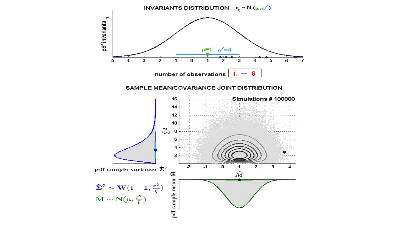
PIC Example 24.12. Sample mean and sample covariance distribution

PIC

Figure 24.10: Video

Consider a normal model (24.39) in the univariate case ¯ı=1. Figure 24.10 shows the joint and marginal distributions of sample mean (24.41) and (co)variance (24.42) as functions of the randomized time series I.

24.5.2 Normal-inverse-Wishart prior distribution
Given the normal model (24.39), we assume that the natural parameters θ follow the conjugate distribution (23.209)

Θ∼Conj(ψ(⋅),ηpri,νpri),(24.43)

where ψ(⋅) is given by (49.421);

ηpri≡(ηpriμvec(ηpriσ))≡(μprivec(σ2pri+μpri(μpri)'));(24.44)

σ2pri is an ¯ıׯı symmetric and positive matrix; and νpri is a positive scalar.

Then, the location and dispersion parameters (M,Σ2) of the conditionally normal i.i.d. variables (24.12), which are equivalent to the natural parameters (M,Σ2)⇔Θ, follow a normal-inverse-Wishart (NIW) distribution 70.11 . More precisely, Σ2 follows an inverse-Wishart distribution (49.118)

(Σ2)−1∼Wishart(νpri,1νpri(σ2pri)−1);(24.45)

and M follows a multivariate normal distribution conditioning on σ2

M|σ2∼N(μpri,1νpriσ2).(24.46)

Note that the general conjugate distribution (23.209) has only one parameter νpri to model the uncertainty of the prior. For the NIW distribution, however, we are able to specify another dispersion parameter tpri for the location M, i.e.

M|σ2∼N(μpri,1tpriσ2),(24.47)

and the posterior would still be the NIW, which we will show in the next section.

The above assumptions imply that the marginal distribution of M is Student t, see [Murphy, 2007]

M∼t(μpri,νpritpri(νpri−¯ı+1)σ2pri,νpri−¯ı+1).(24.48)

Hence the expectation (49.137) reads

E{M}=μpri,(24.49)

and the covariance (49.154) reads

Cv{M}=νpriνpri−21tpriσ2pri.(24.50)

Therefore μpri and tpri represent respectively the statistician’s prior best guess and confidence for the location parameter.
The expectation and the covariance of the inverse-Wishart prior (24.45) read as in (49.121)-(49.122). From the expectation of a Wishart random variable (49.109) it follows that

E{(Σ2)−1}=(σ2pri)−1,(24.51)

and from the covariance (49.110) we have

Cv{(Σ2)−1}=1νpri(I¯ı2+K¯ı,¯ı)((σ2pri)−1⊗(σ2pri)−1).(24.52)

Hence we obtain that σ2pri and νpri respectively represent the statistician’s prior best guess and the confidence for the dispersion parameter.

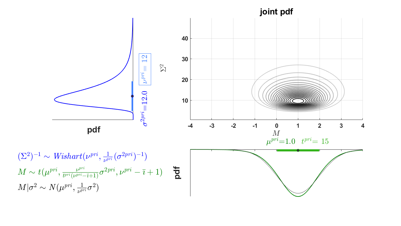
PIC Example 24.13. Normal-inverse-Wishart prior distribution

PIC

Figure 24.11: Video

Consider a univariate i.i.d. variable, conditionally distributed as in (24.12), εt|μ,σ2∼N(μ,σ2) with unknown location and dispersion parameters (μ,σ2). Then we suppose that (Σ2)−1 is univariate Wishart-distributed (24.45), or equivalently gamma (49.112), and M|σ2 is univariate normally distributed (24.47).
In Figure 24.11 we show the joint prior distribution of (M,Σ2) by varying the parameters σ2pri,νpri,μpri,tpri.

PIC Example 24.14. Consider the GARCH residuals (53b.36) of ¯n=60 stocks in the S&P 500.
We assign flexible probabilities by state-time conditioning on the VIX smoothed-scored log-return as in Example 23.4 and we compute the corresponding HFP covariance ˆs2 (24.3). Then, we shrink the HFP covariance to a correlation ˆs2←corr(ˆs2) (10.22) to ensure that the GARCH residuals have unit variance as in (41.76).
We want to regularize the HFP correlation ˆs2←corr(ˆs2) (10.22) so as to have as many null off-diagonal entries as possible [(σ2ε)−1]m,n=0 (21.86) in order to obtain a parsimonious Gaussian Markov random field structure (E.11.31). Then, we perform Bayes estimation under the normal-inverse-Wishart model (Table 24.8) where we set μpri≡0¯n×1,σ2pri≡I¯nׯn and high confidence in the prior tpri,νpri.

24.5.3 Normal-inverse-Wishart posterior distribution
The NIW model (24.47)-(24.45) is conjugate of the normal likelihood (24.40) and thus the posterior (23.172) is also NIW 70.12 , with parameters that can be computed analytically.

The posterior distribution of (Σ2)−1 is Wishart

(Σ2)−1|i∼Wishart(νpos,1νpos(σ2pos)−1),(24.53)

and the conditional posterior distribution of M is normal

M|σ2,i∼N(μpos,1tposσ2).(24.54)

As a result, according to (24.48), the unconditional posterior of M is Student t 70.18 

M|i∼t(μpos,νpostpos(νpos−¯ı+1)σ2pos,νpos−¯ı+1).(24.55)

In the above equations, the posterior expectation μpos reads

μpos=γμμpri+(1−γμ)ˆm,(24.56)

where ˆm is the historical sample mean (24.2) and the parameter γμ∈[0,1] is defined using the confidence parameter for the location prior tpri (24.47) and the sample size ¯t as

γμ≡tpritpri+¯t;(24.57)

the posterior dispersion parameter σ2pos reads

σ2pos=γσσ2pri+(1−γσ)ˆs2+γμ(1−γσ)(μpri−ˆm)(μpri−ˆm)',(24.58)

where ˆs2 is the historical sample covariance (24.4) and the parameter γσ∈[0,1] is defined using the confidence parameter for the dispersion prior νpri (24.45) and the sample size ¯t as

γσ≡νpriνpri+¯t;(24.59)

the parameter tpos is

tpos=tpri+¯t,(24.60)

and νpos is

νpos=νpri+¯t.(24.61)

Refer to [Aitchison and Dunsmore, 1975] for more details.

The interpretation of the posterior parameters in (24.56)-(24.61) is the same as the prior parameters in (24.45)-(24.47), with the substitution pos←pri for all the parameters.

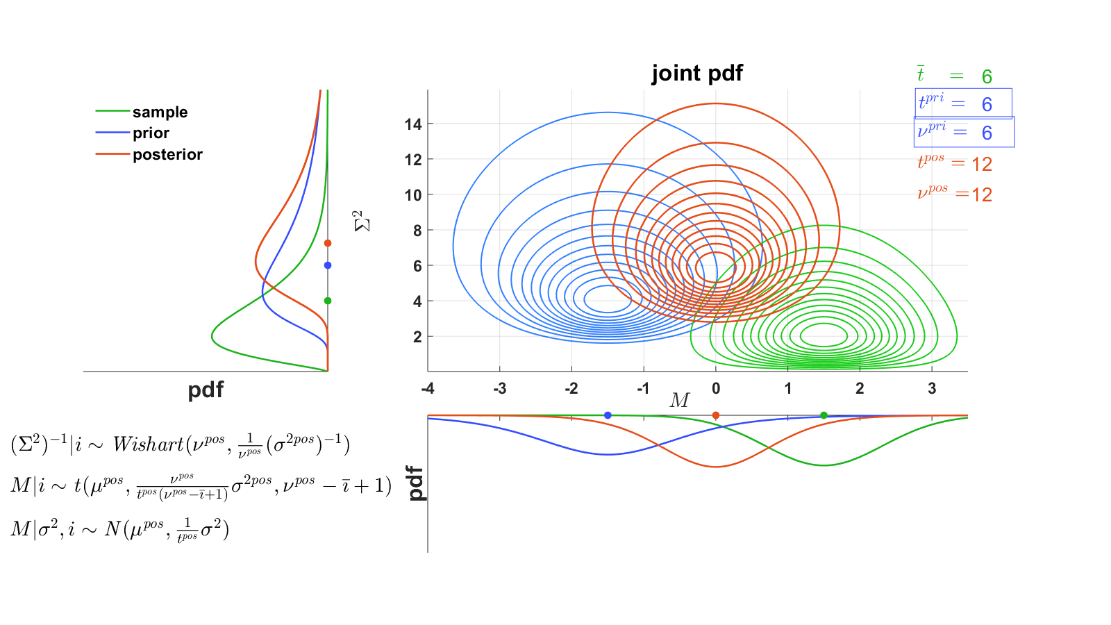
PIC Example 24.15. Normal-inverse-Wishart posterior distribution

PIC

Figure 24.12: Video

We continue from Example 24.13.
In Figure 24.12 we show three distributions:
- the joint prior distribution of (M,Σ2) (24.45)-(24.46), with confidence parameters (νpri,tpri)
- the joint distribution of sample mean and sample variance (ˆM,ˆΣ2) (24.41)-(24.42), with number of observations ¯t
- the joint posterior distribution of (M,Σ2) (24.53)-(24.55).
As we let the confidence in the prior and the number of observations ¯t vary, the posterior shrinks between the prior and the sample.
For a better visualization, we assume knowledge of the true parameters to plot the sample mean and sample variance pdf’s, keeping them fixed as the number of observations varies, similarly to what we do in Figure 24.10 for the frequentist analysis.

PIC Example 24.16. We continue from Example 24.14. We compute the posterior distributions of the conditional location M|i (24.53) and dispersion (Σ2)−1|i (24.55).

24.5.4 Student t predictive distribution

From the normal model (24.12) and the normal-inverse-Wishart posterior (24.53)-(24.54), we can compute the posterior predictive distribution for the future variable εt (23.214), which is t-distributed 70.13 

εt|(ϵ1,…,ϵ¯t)∼t(μpos,tpos+1tposσ2pos,νpos),t>¯t.(24.62)

A word of reflection: the reader should not be puzzled that the i.i.d. variables εt, which are supposed to be independent across time (36.2), appear to be dependent under the posterior predictive distribution (24.62).

Alert 24.1. The variables are only independent conditionally given the knowledge of the parameters (μ,σ2), as shown in Example 24.17.

PIC Example 24.17. Consider two univariate i.i.d. normal variables

ε1|μd=ε2|μ∼N(μ,1), independent(24.63)

where the location parameter is a standard normal random variable

M∼N(0,1).(24.64)

Then the distribution of ε2 conditional on ε1=ϵ1 reads 70.31 

ε2|ϵ1∼N(12ϵ1,32).(24.65)

24.5.5 Classical equivalent, uncertainty and shrinkage

In our normal-inverse-Wishart posterior (24.53)-(24.54), the classical-equivalent (23.173) of the location parameter M is μcl_eq≡E{M}=μpos, as defined in (24.56). According to the shrinkage effect (23.178), if the length ¯t of the time series i≡{ϵ1,…,ϵ¯t} is large, then the parameter μcl_eq shrinks towards the sample mean ˆm; instead, it shrinks towards the prior μpri when it is the confidence tpri in the prior to be large

ˆmlarge dataset ¯t←μcl_eq=μposhigh confidence tpri→μpri.(24.66)

On the other hand, one possible classical-equivalent of the dispersion parameter Σ2 is σ2cl_eq≡σ2pos as defined in (24.58), which satisfies (σ2cl_eq)−1=E{(Σ2)−1}. Similar to the location, the parameter σ2cl_eq shrinks towards the sample covariance ˆs2 if the length ¯t of the time series is large; instead, it shrinks towards the prior σ2pri when the confidence νpri in the prior is large

ˆs2large dataset ¯t←σ2cl_eq=σ2poshigh confidence νpri→σ2pri.(24.67)

The classical-equivalent σ2cl_eq has a slightly more complex expression when defined as the mode (23.174) of the posterior distribution 70.16 -70.14 .

When tpri=νpri, we recover the general shrinkage (23.213) for exponential family

(ˆmvec(ˆs2+ˆmˆm'))ˆηlarge dataset ¯t←(μposvec(σ2pos+μpos(μpos)'))ηposhigh confidence νpri→(μprivec(σ2pri+μpri(μpri)'))ηpri.(24.68)

PIC Example 24.18. In Figure 24.12 we highlight the shrinkage effects (24.66) and (24.67) of the classical equivalent.

PIC Example 24.19. Bayesian estimation: stocks
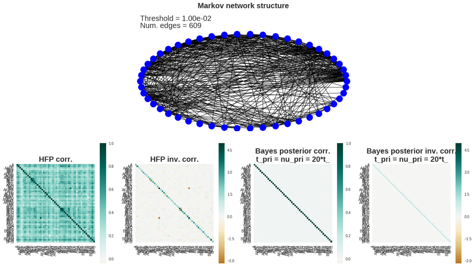
PIC

Figure 24.13:

We continue from Example 24.16. Our regularized estimate for the location and dispersion are the classical-equivalent parameters (23.173), respectively μcl_eq=μpos (24.56) and σ2cl_eq=σ2pos (24.58).
In the bottom plots Figure 24.13 we show:
-) the HFP correlation ˆs2 (24.3)-(10.22) and the corresponding inverse correlation (ˆs2)−1 (left);
-) the Bayes posterior σ2pos (24.58) and the corresponding inverse (σ2pos)−1 (right).
We observe that as the confidence in the prior νpri increases, the off-diagonal terms in the Bayes posterior σ2pos converge to 0 as follows from the shrinkage effect (24.67).
In the top plot of Figure 24.13, we show the Gaussian Markov random field (21.85) structure of the i.i.d. variables (see Section 24.6.5), where the edges are missing if the absolute value of the corresponding entry of the inverse covariance falls below a given threshold (21.86). The more the confidence in the prior νpri increases, the more parsimonious the conditional independence (E.11.31) structure. Refer to Example 24.27 to compare with the glasso regularization.

The posterior of the expectation M is t-distributed (24.55) like the prior (24.48) and hence the uncertainty in the estimate of the expectation, as defined in (23.175), reads

s2μ=νpostpos(νpos−2)σ2pos.(24.69)

It is immediate to verify that the uncertainty (24.69) shrinks to zero in the presence of a long time series or high confidence in the prior, according to the shrinkage effect (23.180).

On the other hand, the posterior of the covariance Σ2 follows an inverse-Wishart distribution (24.53) like the prior (24.45) and then the uncertainty of the covariance estimate, as defined in (23.175), reads similarly to (24.52)

s2σ2=1νpos(I¯ı2+K¯ı,¯ı)((σ2pos)−1⊗(σ2pos)−1),(24.70)

where K¯ı,¯ı is the ¯ı2ׯı2 commutation matrix (43.592). If we choose the modal square-dispersion (23.176) as uncertainty for the posterior distribution of Σ2 we obtain different expressions 70.17 -70.15 . Again, it is immediate to verify that the uncertainty (24.70) and its alternative formulations shrink to zero in the presence of a long time series or high confidence in the prior, according to the shrinkage effect (23.180).

PIC Example 24.20. In Figure 24.12 we highlight the shrinkage effect (23.180) for the uncertainty of location s2μ (24.69) and of dispersion s2σ2 (24.70).

εt|μ,σ2∼N(μ,σ2),
(Σ2)−1∼Wishart(νpri,1νpri(σ2pri)−1);
M|σ2∼N(μpri,1νpriσ2).
(Σ2)−1|i∼Wishart(νpos,1νpos(σ2pos)−1),
M|σ2,i∼N(μpos,1tposσ2).
εt|(ϵ1,…,ϵ¯t)∼t(μpos,tpos+1tposσ2pos,νpos),t>¯t.
I|θ∼f(i|θ).
εt∼F(ε) i.i.d..
i≡(ϵ1,…,ϵt,…,ϵ¯t)≡⎛⎜ ⎜ ⎜ ⎜ ⎜ ⎜ ⎜ ⎜⎝ϵ1,1ϵ1,tϵ1,¯t⋅⋅⋅ϵi,1⋯ϵi,t⋯ϵi,¯t⋅⋅⋅ϵ¯ı,1ϵ¯ı,tϵ¯ı,¯t⎞⎟ ⎟ ⎟ ⎟ ⎟ ⎟ ⎟ ⎟⎠,
fθ(i)=∏¯tt=1fθ(ϵt),
f(ϵ1,…,ϵ¯t|θ)i.i.d.=∏¯tt=1f(ϵt|θ)=e¯t(θ'ˆη−ψ(θ)+lnˆh),
Θ|i∼Conj(¯tψ(⋅),¯tηpos,νpos¯t)=Conj(ψ(⋅),ηpos,νpos),
f(ϵt|ϵ1,…,ϵ¯t)≡∫f(ϵt|θ)fψ(θ|i)dθ(23.214)=g(ηpos,νpos)h(ϵt)g(11+νposτ(ϵt)+νpos1+νposηpos,1+νpos),t>¯t.
εt∼N(μ,σ2).
θ≡(θμvec(θσ))≡⎛⎝(σ2)−1μ−12vec((σ2)−1)⎞⎠.
τ(x)≡(τμ(x)τσ(x))≡(xvec(xx')).
ψ(θμ,θσ)=−14θ'μ(θσ)−1θμ−12lndet(−2θσ).
∑¯tt=1ptlnfθ(ϵt)=θ'μˆηHFPμ+tr(θσˆηHFPσ)−ψ(θ)+lnh(24.16)=−¯ı2ln(2π)−12ln(det(σ2))−12[tr(ˆs2HFPε(σ2)−1)+(ˆmHFPε−μ)'(σ2)−1(ˆmHFPε−μ)].
ˆmHistε≡ˆEHist{ε}=1¯t∑¯tt=1ϵt.
ˆs2Histε≡ˆCvHist{ε}=1¯t∑¯tt=1(ϵt−ˆmHistε)(ϵt−ˆmHistε)'(24.4)=1¯t∑¯tt=1ϵtϵ't−ˆmHistε(ˆmHistε)'.
I≡(ε1,…,εt,…,ε¯t)≡⎛⎜ ⎜ ⎜ ⎜ ⎜ ⎜ ⎜ ⎜⎝ε1,1ε1,tε1,¯t⋅⋅⋅εi,1⋯εi,t⋯εi,¯t⋅⋅⋅ε¯ı,1ε¯ı,tε¯ı,¯t⎞⎟ ⎟ ⎟ ⎟ ⎟ ⎟ ⎟ ⎟⎠.
ˆM|μ,σ2∼N(μ,1¯tσ2),
ˆΣ2|μ,σ2∼Wishart(¯t−1,1¯tσ2).
ˆMmean|μ=esmean(I)|μ≡(1¯t∑¯tt=1εt)|μ∼N(μ,1∕¯t),
Θ∼Conj(¯tψ(⋅),¯tηpri,νpri¯t)=Conj(ψ(⋅),ηpri,νpri),
Σ2∼InvWishart(ν,ψ2)
E{X}=μ,Cv{X}=γσ2,
Cv{X}=νν−2σ2.
E{Σ2}=1ν−¯n−1ψ2,
Cv{[Σ2]m,n,[Σ2]p,q}=2[ψ2]m,n[ψ2]p,q+(ν−¯n−1)([ψ2]m,p[ψ2]n,q+[ψ2]m,q[ψ2]n,p)(ν−¯n)(ν−¯n−1)2(ν−¯n−3).
E{W2}=νσ2,
Cv{W2}=ν(I¯n2+K¯n,¯n)(σ2⊗σ2),
Wishart(ν,σ2)⇔Gamma(ν,σ2)⇔σ2χ2ν.
M|σ2∼N(μpri,1tpriσ2),
ϵd,t=xd,t−xd,t−1−μσt−1,
ˆs2HFPε≡ˆCvHFP{ε}=∑¯tt=1pt(ϵt−ˆmHFPε)(ϵt−ˆmHFPε)'(24.3)=∑¯tt=1ptϵtϵ't−ˆmHFPε(ˆmHFPε)'.
corr(σ2)≡Diag(1¯n×1vol(σ2))×σ2×Diag(1¯n×1vol(σ2)),
E{εt}=0,   Sd{εt}=1,
[(σ2)−1]m,n=0⇔(m∼n)∉E.
(Ym⊥⊥Yn)|Y−{m,n}⇔[(σ2)−1]m,n=0.
f(i|θ)=exp(¯t(θ'μˆημ+tr(θσˆησ)−ψ(θ)+lnh))(24.40)=(2π)−¯ı¯t2det(σ2)−¯t2exp(−¯t2[tr(ˆs2(σ2)−1)+(ˆm−μ)'(σ2)−1(ˆm−μ)]),
fpos(θ)≡f(θ|i)=f(i|θ)fpri(θ)∫f(i|ϑ)fpri(ϑ)dϑ,
M∼t(μpri,νpritpri(νpri−¯ı+1)σ2pri,νpri−¯ı+1).
μpos=γμμpri+(1−γμ)ˆm,
νpos=νpri+¯t.
M|i∼t(μpos,νpostpos(νpos−¯ı+1)σ2pos,νpos−¯ı+1).
ˆθmean≡∫θfpos(θ)dθ.
ˆθclassicallow confidence←ˆθbayesposteriorhigh confidence→θpriprior.
σ2pos=γσσ2pri+(1−γσ)ˆs2+γμ(1−γσ)(μpri−ˆm)(μpri−ˆm)',
ˆθmp≡argmaxθfpos(θ).
Shrinkage:1¯t∑¯tt=1τ(ϵt)(23.208)=ˆηlarge dataset ¯t←ηposhigh confidence νpri→ηpri.
ˆmlarge dataset ¯t←μcl_eq=μposhigh confidence tpri→μpri.
ˆs2large dataset ¯t←σ2cl_eq=σ2poshigh confidence νpri→σ2pri.
Y∼N(μ,σ2),
s2θ≡∫(θ−ˆθmean)(θ−ˆθmean)'fpos(θ)dθ.
s2μ=νpostpos(νpos−2)σ2pos.
s2θhigh confidence→0.
Cv{(Σ2)−1}=1νpri(I¯ı2+K¯ı,¯ı)((σ2pri)−1⊗(σ2pri)−1).
K¯¯¯m,¯n≡∑m,n[δ(m)¯¯¯m×1(δ(n)¯n×1)']⊗[δ(n)¯n×1(δ(m)¯¯¯m×1)'].
s2θ≡(−∇2θ,θlnfpos(θ)|θ=ˆθmp)−1.
s2σ2=1νpos(I¯ı2+K¯ı,¯ı)((σ2pos)−1⊗(σ2pos)−1),

Bibliography


External Links


Discussions


arpm small logo
About us Start here
Clients and partners Corporate program Academia program
Contact us Events Book
Contact us   Linkedin
Terms ⚪ Privacy policy ⚪ Refund policy ⚪ Cookies policy ⚪ Copyright ⚪ IT requirements
© 2026 ARPM, All rights reserved.