Lab | Supervised learning: classification

Chapter 19
Supervised learning: classification

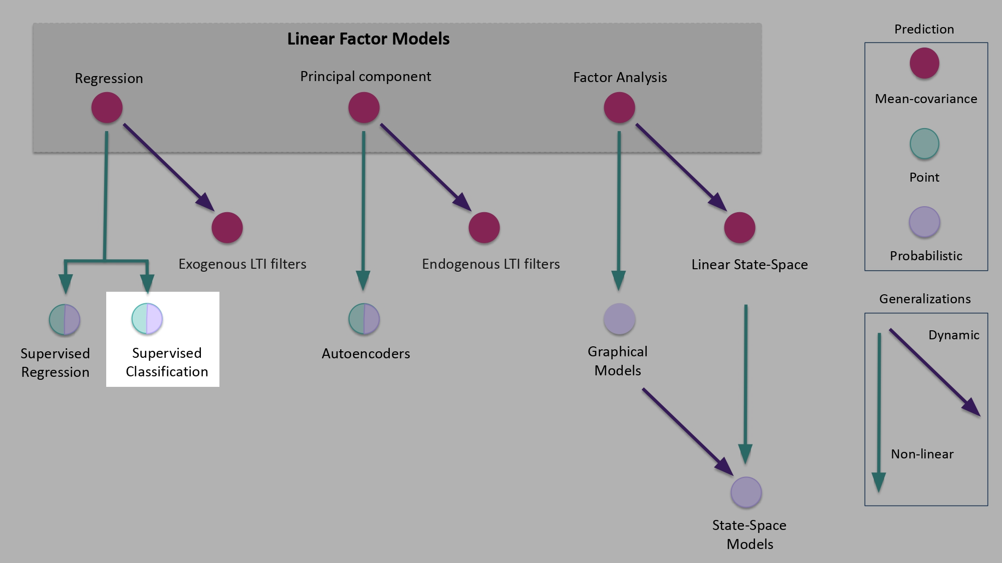
In the present chapter we discuss the main supervised classification models for both point (17.49) and probabilistic (17.74) prediction, where the goal is to predict either the specific outcome and/or the conditional probability of some categorical (17.9) target variables, or outputs (17.3), given the outcome of some continuous factors, or inputs (17.4), see Section 17.1.1 and Section 17.2. Supervised classification is a generalization of regression linear factor models with categorical outputs (17.9), as shown in Figure 1.6 which we report in highlight in the below

The aim for both point and probabilistic prediction is either for stress-testing (17.13) or forecasting (17.16).

Intuition We continue from the example described in the Supervised learning: regression Intuition. In our case, suppose we are not interested in the details of the portfolio return

R_{t_{n o w} \to t_{n o w} + 1}

(14.1), but more simply in whether the return will be positive or negative

X^{b i n a r y} \equiv {\begin{matrix} 1 & if R_{t_{n o w} + 1} > 0 0 & if R_{t_{n o w} + 1} < 0 . \end{matrix}

(19.1)

Also, let us use as input, the same return on the S&P 500 index (14.2), but between yesterday and today, so that we obtain a predictive model

z \equiv r_{S & P, t_{n o w}} .

(19.2)

Then, the conditional predictive distribution is Bernoulli

X^{b i n a r y} | z \sim B e r n o u l l i (p_{β^{l o g i t}}^{l o g i t} (1 | z));

(19.3)

and we can use a binary classification model based on logistic regression with interactions to parametrize the conditional probability of the positive outcome

p_{b} (1 | z) = \frac{e_{0}^{b_{0} + b_{1} z + b_{2} z^{2}}}{1 + e_{0}^{b_{0} + b_{1} z + b_{2} z^{2}}},

(19.4)

so that $p_{b} (0 | z) = 1 - p_{b} (1 | z)$ . To set the optimal parameters, we should maximize the likelihood with respect to the true distribution

(β_{0}^{l o g i t}, β_{1}^{l o g i t}, β_{2}^{l o g i t}) \equiv argmax b E {ln p_{b} (X | Z)} .

(19.5)

In our case, the realized time series of the output (19.1)

x_{t + 1}^{b i n a r y} = 1_{r_{t + 1} > 0}

(19.6)

joined with the time series of the input (19.2)

z_{t} = r_{S & P, t}

(19.7)

follows from the original time series (14.8)-(19.6)

\begin{matrix} t : & 1 & 2 & 3 & 4 & 5 & 6 & 7 & 8 & 9 - ------ - & - ---- - & - ------ - & - ------- - & - ------- - & - ----- - & - ----- - & - ------- - & - ------- - & - ------- - x_{t + 1}^{b i n a r y} : & 0 & 1 & 0 & 1 & 1 & 0 & 1 & 0 & 0 z_{t} : & 0.4 % & - 0.3 % & - 0.19 % & - 0.72 % & 0.31 % & 1.39 % & - 0.28 % & - 0.49 % & - 0.16 % \end{matrix}

(19.8)

Then, if the output $X_{t + 1}^{b i n a r y}$ is conditionally i.i.d. across time given the input $Z_{t} = z$ , and if the input $Z_{t}$ is i.i.d., we can fit the conditional probability $p (z)$ (19.4) by replacing the true random variables in (19.5) with their sample counterparts in the time series (19.8), using the optimal parameters (19.5) which read

(β_{0}^{l o g i t}, β_{1}^{l o g i t}, β_{2}^{l o g i t}) \approx (- 0.11, - 163.72, - 1.06) .

(19.9)

In our case the predicted conditional probability (19.4) that portfolio return $x_{¯ t + 1}^{b i n a r y}$ (19.1) will be positive tomorrow reads

z_{¯ t} = 0.37 % \Rightarrow p_{β^{l o g i t}}^{l o g i t} (1 | z_{¯ t}) \approx 54 %,

(19.10)

to be compared with the unconditional estimated probability $p \approx 44 %$ . From the probabilistic prediction (19.10), we can naturally obtain a point prediction for the future outcome of the binary variable (19.1)

z_{¯ t} = 0.37 % \Rightarrow {¯ x}^{b i n a r y} = 1_{p_{β^{l o g i t}}^{l o g i t} (1 | z_{¯ t}) > 0.5} = 1 .

(19.11)

In point prediction (17.49), the predictor, or classifier (17.51) is given by a sum of indicators function on a suitable partition $Δ (R^{¯ k}) \equiv {Z^{(c)}}_{c = 1}^{(c)}$ (44.132) of the input domain $R^{¯ k}$

¯ x \equiv c_{Δ} (z) \equiv \sum_{c = 1}^{¯ c} c 1_{z \in Z^{(c)}}^{(c)};

(19.12)

and in probabilistic prediction (17.74), the predictor (17.75) is given by (conditional) probabilities

X | z \sim ¯ p (x | z) .

(19.13)

Theory Point prediction is but an instance of decision theory (Table 6.4), as summarized in the below

The true outcome $x$ (17.49) of the output $X$ (17.3) is the state (6.7), which we predict via the realization $z$ of the input random vector $Z$ (17.4), i.e. the observed input (6.89), by means of a predictor $¯ x \equiv c_{Δ} (\cdot)$ (17.50), as identified by the partition $Δ (R^{¯ k})$ , which is the decision (6.91).
To evaluate the goodness of the prediction, we consider a divergence $D (x ∥ ¯ x)$ (43.269), which is the loss (6.14). Then, by feeding the loss with the data generating process (DGP) $f_{X, Z}$ (6.111) we obtain the error $E^{f} {D (X ∥ c_{Δ} (Z))}$ (17.71), which is the Bayes risk of a decision (6.118). Note from Table 19.1 that a decision in this context is a predictor $c_{Δ}$ .
The search for the optimal predictor is performed across parametric functions, as summarized in the table below for point prediction (17.49)

Similar to the point counterpart (Table 19.1), also probabilistic prediction is but an instance of decision theory (Section 6.1), see Table 17.5 and also the below

The true outcome $x$ (17.49) of the output $X$ (17.3) is the state (6.7), which we predict via the realization $z$ of the input random vector $Z$ (17.4), i.e. the observed input (6.89), by means of a predictor $¯ p (\cdot | \cdot)$ (17.75), which is the decision (6.91).
To evaluate the goodness of the prediction, we consider a scoring rule $s . r u l e ({x, z}, ¯ p (\cdot | \cdot))$ (17.95), which is the negative counterpart of a loss (6.14). Then, evaluating the expected loss, with the data generating process (DGP) $f_{X, Z}$ (6.111) we obtain the error $E^{f} {- s . r u l e ({X, Z}, ¯ p (\cdot | \cdot))}$ (17.97), which is the Bayes risk of a decision (6.118). Note from Table 19.3 that a decision in this context is a predictor $¯ p$ .
The search for the optimal predictor is performed across parametric functions, as summarized in the table below for probabilistic prediction (17.74)

The evaluation and optimization components in Tables 19.1-19.4 correspond to the frequentist approach (Section 6.3.4) discussed in general decision theory, see Table 6.4.

Most notable errors for supervised classification are e.g. the misclassification error (12.71) in point prediction (17.49); or the cross-entropy (5.5) in probabilistic prediction (17.74).

Practice The main classes of supervised classification models for both point (17.49) and probabilistic prediction (17.74) are summarized in the table bellow

In order to find an optimal prediction, the standard approach is to restrict the search to a parametric family of predictors such as linear bases, trees, or neural networks:

γ_{ϑ} (z) = ⎧ ⎪ ⎪ ⎪ ⎪ ⎪ ⎨ ⎪ ⎪ ⎪ ⎪ ⎪ ⎩ \begin{matrix} basis-linear & b ϕ (z) & ϑ = b trees & β_{Δ} ϕ_{Δ}^{1 h o t} (z) & ϑ = Δ neural networks & n n_{ϑ} (z) & ϑ = {b^{(1)}, \dots, b^{(¯ l)}} gradient boosting & . . . & . . . \end{matrix}

(19.14)

The remainder of this chapter is organized as follows.

In Section 19.1 we discuss point classification models for binary output variables.

In Section 19.2 we extend binary point classification to the multinomial case.

In Section 19.3 we present the more ambitious probabilistic classification models based on different errors, such as cross-entropy, Gini impurity and probabilistic misclassification.

Finally, in Section 19.4 we address some points of interest.

¯ ¯ ¯ x \approx x .

¯ f (x) \approx f (x) .

X \in {x^{(1)}, \dots, x^{(¯ c)}} \Leftrightarrow X \in {1, \dots, ¯ c},

X \equiv ⎛ ⎜ ⎜ ⎝ \begin{matrix} X_{1} ⋮ X_{¯ n} \end{matrix} ⎞ ⎟ ⎟ ⎠,

Z \equiv ⎛ ⎜ ⎜ ⎝ \begin{matrix} Z_{1} ⋮ Z_{¯ k} \end{matrix} ⎞ ⎟ ⎟ ⎠,

t > t_{n o w}, s > t_{n o w} .

t > t_{n o w}, s \leq t_{n o w} .

X \equiv w_{1, t_{n o w}} R_{1, t_{n o w} + 1} + w_{2, t_{n o w}} R_{2, t_{n o w} + 1},

Z \equiv R_{S & P, t_{n o w} + 1} .

X^{b i n a r y} \equiv {\begin{matrix} 1 & if R_{t_{n o w} + 1} > 0 0 & if R_{t_{n o w} + 1} < 0 . \end{matrix}

z \equiv r_{S & P, t_{n o w}} .

\begin{matrix} t : & 1 & 2 & 3 & 4 & 5 & 6 & 7 & 8 & 9 & 10 - -- - & - ----- - & - ------- - & - ------- - & - ------- - & - ----- - & - ----- - & - ------- - & - ------- - & - ------- - & - ------- - x_{t} : & 0.29 % & - 0.66 % & 0.16 % & - 0.29 % & 0.28 % & 1.5 % & - 0.95 % & 0.31 % & - 0.18 % & - 0.24 % z_{t} : & 0.4 % & - 0.3 % & - 0.19 % & - 0.72 % & 0.31 % & 1.39 % & - 0.28 % & - 0.49 % & - 0.16 % & 0.37 % \end{matrix}

x_{t + 1}^{b i n a r y} = 1_{r_{t + 1} > 0}

p_{b} (1 | z) = \frac{e_{0}^{b_{0} + b_{1} z + b_{2} z^{2}}}{1 + e_{0}^{b_{0} + b_{1} z + b_{2} z^{2}}},

(β_{0}^{l o g i t}, β_{1}^{l o g i t}, β_{2}^{l o g i t}) \equiv argmax b E {ln p_{b} (X | Z)} .

\begin{matrix} t : & 1 & 2 & 3 & 4 & 5 & 6 & 7 & 8 & 9 - ------ - & - ---- - & - ------ - & - ------- - & - ------- - & - ----- - & - ----- - & - ------- - & - ------- - & - ------- - x_{t + 1}^{b i n a r y} : & 0 & 1 & 0 & 1 & 1 & 0 & 1 & 0 & 0 z_{t} : & 0.4 % & - 0.3 % & - 0.19 % & - 0.72 % & 0.31 % & 1.39 % & - 0.28 % & - 0.49 % & - 0.16 % \end{matrix}

z_{¯ t} = 0.37 % \Rightarrow p_{β^{l o g i t}}^{l o g i t} (1 | z_{¯ t}) \approx 54 %,

¯ ¯ ¯ x \equiv χ (z) .

Δ (X) \equiv {X^{(j)}}_{j = 1}^{(j)} such that {\begin{matrix} ⋃_{j = 1}^{¯ ȷ} X^{(j)} = X X^{(j)} \cap X^{(j^{'})} = \emptyset & for j \neq j^{'} \end{matrix},

¯ f (X | Z) \approx f (X | Z);

s \in S,

x \in X,

¯ ¯¯ ¯ X \equiv χ (Z) \approx X;

d : x \in X \mapsto a = d (x) \in A .

D (\cdot ∥ \cdot) : {x, y} \in X \times X \mapsto D (x ∥ y) \geq 0,

ℓ : {s \in S, a \in A} \mapsto ℓ (s, a) \in R .

f (x, s) \equiv f (x | s) f (s) .

E^{f} {D (X ∥ ¯ ¯¯ ¯ X)} .

¯ ϱ (f_{S, X}, d) \equiv E {r (S, d)} = E {ℓ (S, d (X))},

s . r u l e (x, ¯ f) \equiv ln ¯ f (x) .

D_{s . r u l e} (f ∥ ¯ f) \equiv E^{f} {- s . r u l e (X, ¯ f)} - H_{s . r u l e} (f) .

E r r o r {X, Y} \equiv P {X \neq Y} = E {D_{01} (X ∥ Y)} .

H (f | | ¯ f) \equiv E^{f} {- ln ¯ f (X)} = - \int f (x) ln ¯ f (x) d x .

Decision theory	Point prediction	Frequentist

State	Output	$x$
Observed input	Input	$z$
DGP	DGP	$f_{X, Z}$
Action	Prediction	$¯ x$
Loss function	Divergence	$D (x ∥ ¯ x)$
Decision	Predictor	$Δ (R^{¯ k}) \Leftrightarrow c_{Δ} (z) : z \mapsto ¯ x \equiv c_{Δ} (z)$
Bayes risk	Error	$E^{f} {D (X ∥ c_{Δ} (Z))}$
Optimization	Optimization	$Δ^{*} \equiv argmin Δ E^{f} {D (X ∥ c_{Δ} (Z))}$

Decision theory	Point prediction	Frequentist

Decision	Predictor	$ϑ \Leftrightarrow ¯ x \equiv c_{Δ_{ϑ}} (z)$
Evaluation	Error	$e r r o r (ϑ, f) \equiv E^{f} {D (X ∥ c_{Δ_{ϑ}} (Z))}$
Optimization	Optimization	$θ \equiv argmin ϑ e r r o r (ϑ, f)$

Decision theory	Probabilistic prediction	Frequentist

State	Output	$x$
Observed input	Input	$z$
DGP	DGP	$f_{X, Z}$
Action	Prediction	$¯ p (\cdot)$
Loss function	Negative scoring rule	$- s . r u l e (x, ¯ p (\cdot))$
Decision	Predictor	$¯ p (\cdot \| \cdot) : z \mapsto ¯ p (\cdot) \equiv ¯ p (\cdot \| z)$
Evaluation	Error	$E^{f} {- s . r u l e (X, ¯ p (\cdot \| Z))}$
Optimization	Optimization	${¯ p}^{*} (\cdot \| \cdot) \equiv argmin ¯ p (\cdot \| \cdot) E^{f} {- s . r u l e (X, ¯ p (\cdot \| Z))}$

Decision theory	Probabilistic prediction	Frequentist

Decision	Predictor	$ϑ \Leftrightarrow ¯ p (\cdot \| \cdot) \equiv p_{ϑ} (\cdot \| \cdot)$
Evaluation	Error	$e r r o r (ϑ, f) \equiv E^{f} {- s . r u l e (X, p_{ϑ} (\cdot \| Z))}$
Optimization	Optimization	$θ \equiv argmin ϑ e r r o r (ϑ, f)$

Chapter 19
Supervised learning: classification

Bibliography

External Links

Discussions

Chapter 19Supervised learning: classification

Bibliography

External Links

Discussions

Chapter 19
Supervised learning: classification