Lab | Maximum likelihood

24.2 Maximum likelihood

Key points

The maximum likelihood with flexible probabilities estimators of the mean and covariance under normality (24.12) coincide with the historical with flexible probabilities estimators (24.18).
The maximum likelihood with flexible probabilities estimators of the location and dispersion parameters of a Student $t$ distribution (24.19) with given degrees of freedom $ν$ can be computed by means of the recursive routine in Table 24.1.

In this section we discuss how to estimate the location and dispersion of the distribution of i.i.d. variables by applying the maximum likelihood approach introduced in Section 23.4. We consider two parametric assumptions: normal (Section 24.2.1) and Student $t$ (Section 24.2.2).

24.2.1 Normal assumption

In this section we apply the maximum likelihood approach for exponential family distributions introduced in Section 23.4.5 to the special case of the multivariate normal (49.1)

ε_{t} \sim N (μ, σ^{2}) .

(24.12)

The standard parameters are $μ$ ( $¯ ı$ -dimensional expected value) and $σ^{2}$ ( $¯ ı \times ¯ ı$ positive definite and symmetric covariance matrix), which are the most important properties of location and dispersion (Section 8).

The multivariate normal is an exponential family distribution with natural parameters $θ \equiv (θ_{μ}, θ_{σ})$ (49.413), features $τ (x)$ (49.417) and log-partition function $ψ (\cdot)$ (49.421). The natural parameters are in one-to-one correspondence with the standard parameters $θ \equiv (θ_{μ}, θ_{σ}) \Leftrightarrow (μ, σ^{2})$ . Our goal is to estimate $θ$ and therefore $(μ, σ^{2})$ .

Given a realized time series $i \equiv {ϵ_{1}, \dots, ϵ_{¯ t}}$ consider the historical mean with flexible probabilities (24.1)

{ˆ m}_{ε}^{H F P} \equiv \sum_{t = 1}^{¯ t} p_{t} ϵ_{t},

(24.13)

and the historical covariance matrix with flexible probabilities (24.3)

{ˆ s}_{ε}^{2 H F P} \equiv \sum_{t = 1}^{¯ t} p_{t} ϵ_{t} ϵ_{t}^{'} - {ˆ m}_{ε}^{H F P} {ˆ m}_{ε}^{H F P'} .

(24.14)

Then the historical with flexible probabilities (HFP) sample features (23.80) read as follows

{ˆ η}_{ϵ}^{H F P} \equiv (\begin{matrix} {ˆ η}_{μ}^{H F P} v e c ({ˆ η}_{σ}^{H F P}) \end{matrix}) = (\begin{matrix} {ˆ m}_{ε}^{H F P} v e c ({ˆ s}_{ε}^{2 H F P} + {ˆ m}_{ε}^{H F P} {ˆ m}_{ε}^{H F P'}) \end{matrix}) .

(24.15)

From the one-to-one correspondence $θ \Leftrightarrow (μ, σ^{2})$ (49.413), the log-likelihood with flexible probabilities (23.79) reads 70.2

\begin{matrix} \sum_{t = 1}^{¯ t} p_{t} ln f_{θ} (ϵ_{t}) & = θ_{μ}^{'} {ˆ η}_{μ}^{H F P} + tr (θ_{σ} {ˆ η}_{σ}^{H F P}) - ψ (θ) + ln h & (24.16) = - \frac{¯ ı}{2} ln (2 π) - \frac{1}{2} ln (det (σ^{2})) - \frac{1}{2} [tr ({ˆ s}_{ε}^{2 H F P} {(σ^{2})}^{- 1}) + {({ˆ m}_{ε}^{H F P} - μ)}^{'} {(σ^{2})}^{- 1} ({ˆ m}_{ε}^{H F P} - μ)] . \end{matrix}

We could proceed to maximize the likelihood, as in (23.67). However, it is easier to leverage the general results for exponential family variables from Section 23.4.5. The gradient of the log-partition is (5.68). Then the maximum likelihood estimates of the natural parameters (23.82) follow from inverting the gradient 70.37

{ˆ θ}^{M L F P} \equiv ⎛ ⎜ ⎝ \begin{matrix} {ˆ θ}_{μ}^{M L F P} v e c ({ˆ θ}_{σ}^{M L F P}) \end{matrix} ⎞ ⎟ ⎠ = ⎛ ⎜ ⎝ \begin{matrix} {({ˆ s}_{ε}^{2 H F P})}^{- 1} {ˆ m}_{ε}^{H F P} - \frac{1}{2} v e c ({({ˆ s}_{ε}^{2 H F P})}^{- 1}) \end{matrix} ⎞ ⎟ ⎠ .

(24.17)

By expressing the standard parameters in terms of the canonical parameters (49.417), we obtain that the maximum likelihood estimates of the location and dispersion for normal variables are the historical mean and historical covariance with flexible probabilities (24.13)-(24.14)

{ˆ μ}_{ε}^{M L F P} = {ˆ m}_{ε}^{H F P}, {ˆ σ}_{ε}^{2 M L F P} = {ˆ s}_{ε}^{2 H F P},

(24.18)

which also follows from the limit of maximum likelihood under Student $t$ assumptions (24.24).

It is comforting to see that we obtain the “same” estimates using two completely different principles, namely the historical and maximum likelihood. However, keep in mind that the assumptions of the maximum likelihood approach, being parametric (23.59), are more restrictive.

24.2.2 Student $t$ assumption

In this section we apply the maximum likelihood approach to estimate location and dispersion under the Student $t$ distribution assumption.

Let us assume as parametric specification (23.59) for the i.i.d. variables $ε_{t} = {(ε_{1, ¯ t}, \dots, ε_{¯ ı, ¯ t})}_{1, ¯ t}^{'}$ a Student $t$ distribution

ε_{t} \sim f_{ε} \in {f_{μ, σ^{2}, ν}^{t}}_{(μ, σ^{2}, ν) \in Θ}^{2},

(24.19)

where the pdf reads (49.144)

f_{μ, σ^{2}, ν}^{t} (x) \equiv \frac{Γ ((ν + ¯ ı) ∕ 2)}{Γ (ν ∕ 2) {(ν π)}^{¯ ı ∕ 2} det {(σ^{2})}^{1 ∕ 2}} {(1 + \frac{{(x - μ)}^{'} {(σ^{2})}^{- 1} (x - μ)}{ν})}^{- (ν + ¯ ı) ∕ 2} .

(24.20)

In this context $Θ$ is the space of parameters $θ \equiv (μ, σ^{2}, ν)$ , where $μ$ is a $¯ ı$ -dimensional location vector; $σ^{2}$ is the $¯ ı \times ¯ ı$ positive definite and symmetric dispersion matrix; and $ν$ is a positive scalar representing the degrees of freedom, which determine the thickness of the tails. Notice the power law decay in the tails, determined by the degrees of freedom $ν$ .

When $ν \to \infty$ the power law becomes an exponential decay, and the Student $t$ becomes the normal distribution $N (μ, σ^{2})$ (49.1). As $ν$ decreases, the tails become thicker and the probability of extreme scenarios increases. When $ν = 1$ the Student $t$ becomes the Cauchy distribution $C a u c h y (μ, σ^{2})$ (49.164), whose tails are so thick that neither expected values nor covariances are defined, and yet the location and dispersion parameters $(μ, σ^{2})$ are always well defined.

Example 24.2. Location-dispersion: MLFP ellipsoid

Let us consider the same setting as in Example 24.1.
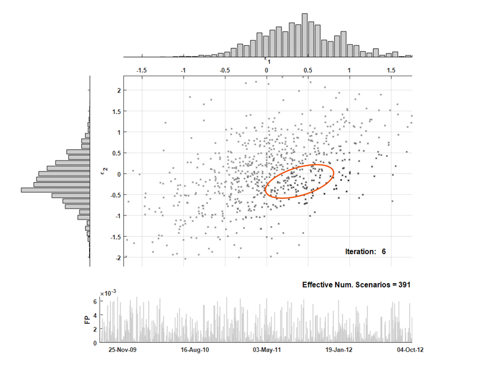
In Figure 24.2 we show the realized residuals ${ϵ_{t} = {(ϵ_{1, t}, ϵ_{2, t})}^{'}}_{t}^{'}$ of a GARCH $(1, 1)$ (41.75)-(41.77) fit of two stocks’ returns. We overlay the ellipsoid $\partial E ({ˆ m}_{ε}^{M L F P}, {ˆ s}_{ε}^{2 M L F P})$ (8.45) defined by the MLFP estimates of location ${ˆ μ}_{ε}^{M L F P}$ (24.21) and dispersion ${ˆ σ}_{ε}^{2 M L F P}$ (24.22), computed with the routine in Table 24.1, with $ν = 4$ .
We also plot the respective flexible probabilities ${p_{t}}_{t}^{¯ t}$ and display the effective number of scenarios $ˆ t \equiv e n s (p_{1}, \dots, p_{¯ t})$ (23.21).

The Student $t$ distribution does not belong to the exponential family (49.395), unless $ν \to \infty$ (24.12). Hence, we cannot leverage the general results in Section 23.4.5. However, we can explicitly perform the maximum likelihood with flexible probabilities (MLFP) optimization (23.67), obtaining the MLFP parameter ${ˆ μ}_{ε}^{M L F P}$ as the solution of the following implicit equation 70.4

{ˆ μ}_{ε}^{M L F P} = \sum_{t = 1}^{¯ t} \frac{p_{t} w_{t}}{\sum_{s = 1}^{¯ t} p_{s} w_{s}} ϵ_{t},

(24.21)

and the MLFP parameter ${ˆ σ}_{ε}^{2 M L F P}$ as the solution of

{ˆ σ}_{ε}^{2 M L F P} = \sum_{t = 1}^{¯ t} p_{t} w_{t} (ϵ_{t} - {ˆ μ}_{ε}^{M L F P}) {(ϵ_{t} - {ˆ μ}_{ε}^{M L F P})}_{t}^{'},

(24.22)

with weights defined as

w_{t} = \frac{(ν + ¯ ı)}{ν + {(ϵ_{t} - {ˆ μ}_{ε}^{M L F P})}_{t}^{'} {({ˆ σ}_{ε}^{2 M L F P})}^{- 1} (ϵ_{t} - {ˆ μ}_{ε}^{M L F P})} .

(24.23)

Note that the scatter matrix estimator (24.22) is purposely not normalized by $\sum_{s = 1}^{¯ t} p_{s} w_{s}$ because $σ_{ε}^{2}$ is not the covariance (49.154). On the other hand, the location vector estimator (24.21) is normalized, because $μ_{ε}$ is the expectation (49.153), when the expectation is properly defined ( $ν > 1$ ).

In theory, to calibrate the degrees of freedom $ν$ , we should compute a solution $({ˆ μ}_{ε}^{M L F P}, {ˆ σ}_{ε}^{2 M L F P})$ for each value of $ν > 0$ , then compute the respective likelihood, and finally choose the degrees of freedom $ν_{ε}^{M L F P}$ that give rise to the highest likelihood (23.67). In reality, we recommend using a small number of degrees of freedom, such as $ν \approx 4$ , regardless of the fit, for robustness (for a detailed discussion on robustness, see Section 23.7).

Similarly, it is possible to perform the MLFP optimization under the most general multivariate elliptical assumption, which include the Student $t$ (24.19) as a special case 70.3 .

The MLFP parameters ${ˆ μ}_{ε}^{M L F P}$ and ${ˆ σ}_{ε}^{2 M L F P}$ depend on the assumption we make on the degrees of freedom.

In the normal case ( $ν \to \infty$ ) the weights (24.23) become constant, $w_{t} = 1$ , and $({ˆ μ}_{ε}^{M L F P}, {ˆ σ}_{ε}^{2 M L F P})$ assume the same expression than the historical with flexible probabilities (HFP) mean (24.1) and covariance (24.3)

{ˆ μ}_{ε}^{M L F P} = {ˆ m}_{ε}^{H F P}, {ˆ σ}_{ε}^{2 M L F P} = {ˆ s}_{ε}^{2 H F P} .

(24.24)

This follows also from a direct maximization of the normal likelihood (24.18).

In the general case of finite degrees of freedom $ν ≪ \infty$ , the weights (24.23) depend on ${ˆ μ}_{ε}^{M L F P}$ and ${ˆ σ}_{ε}^{2 M L F P}$ via the Mahalanobis distance $M a h_{{ˆ σ}_{ε}^{2 M L F P}}^{2} (ϵ_{t}, {ˆ μ}_{ε}^{M L F P})$ (43.185). Hence, extreme scenarios, i.e. observations $ϵ_{t}$ with large Mahalanobis distance, $M a h_{{ˆ σ}_{ε}^{2 M L F P}}^{2} (ϵ_{t}, {ˆ μ}_{ε}^{M L F P}) ≫ ¯ ı$ , have a negligible weight, $w_{t} ≪ 1$ , in the estimation. This result is intuitive: with low degrees of freedom $ν ≪ \infty$ , the tails are thick and thus we expect to see several extreme scenarios. If we did not down-weight such scenarios, i.e. if we set $w_{t} \approx 1$ , the MLFP parameters $({ˆ μ}_{ε}^{M L F P}, {ˆ σ}_{ε}^{2 M L F P})$ would be the same as the HFP estimates $({ˆ m}_{ε}^{H F P}, {ˆ s}_{ε}^{2 H F P})$ and thus the ensuing ellipsoid would be spuriously stretched out to account for such scenarios, as we saw in the case of the geometrical interpretation (24.11).

The MLFP formulas (24.21)-(24.22)-(24.23) are a system of implicit equations for ${ˆ μ}_{ε}^{M L F P}$ and ${ˆ σ}_{ε}^{2 M L F P}$ , which appear difficult to solve. In reality, the following simple recursion quickly converges to a solution, see Figure 24.2.

Let us denote with $˜ μ$ and ${˜ σ}^{2}$ the location and dispersion parameters respectively obtained in the previous iteration. Convergence in the above routine occurs when the maximum relative norm [W] between two subsequent updates $(˜ μ, μ)$ and $({˜ σ}^{2}, σ^{2})$ are smaller than a required threshold

max {∥ ˜ μ - μ ∥_{\infty} ∕ ∥ ˜ μ ∥_{\infty}, ∥ {˜ σ}^{2} - σ_{\infty}^{2} ∥ ∕ ∥ {˜ σ}_{\infty}^{2} ∥} < ξ .

(24.25)

Example 24.3. Consider as i.i.d. variables $ε_{t}$ two different zero swap rates (65.45), and exponential decay flexible probabilities $p_{t}$ (23.6) with half-life $τ_{H L} = 180$ .
By setting $ν = 5$ , we apply maximum likelihood routine in Table 24.1, obtaining the MLFP estimates of location (24.21) and dispersion (24.22)

{ˆ μ}_{ε}^{M L F P} = 1 0^{- 4} \times (\begin{matrix} - 0.14 - 0.29 \end{matrix}), {ˆ σ}_{ε}^{2 M L F P} = 1 0^{- 6} \times (\begin{matrix} 0.06 & 0.08 0.08 & 0.23 \end{matrix}) .

(24.26)

Example 24.4. Consider as i.i.d. variable $ε_{t}$ the equity compounded return of Cisco Systems (CSCO), and exponential decay flexible probabilities $p_{t}$ (23.6) with half-life $τ_{H L} = 800$ .
Since we are concerned of extreme outcomes we apply maximum likelihood routine in Table 24.1 assuming a Cauchy distribution (49.164), namely $ν = 1$ , obtaining the MLFP estimates of location (24.21) and dispersion (24.22)

{ˆ μ}_{ε}^{M L F P} = 1 0^{- 5} \times 9.7, {ˆ σ}_{ε}^{2 M L F P} = 1 0^{- 3} \times 9.1 .

(24.27)

ε_{t} \sim N (μ, σ^{2}) .

{ˆ μ}_{ε}^{M L F P} = {ˆ m}_{ε}^{H F P}, {ˆ σ}_{ε}^{2 M L F P} = {ˆ s}_{ε}^{2 H F P},

ε_{t} \sim f_{ε} \in {f_{μ, σ^{2}, ν}^{t}}_{(μ, σ^{2}, ν) \in Θ}^{2},

X \sim N (μ, σ^{2}),

θ \equiv (\begin{matrix} θ_{μ} v e c (θ_{σ}) \end{matrix}) \equiv ⎛ ⎝ \begin{matrix} {(σ^{2})}^{- 1} μ - \frac{1}{2} v e c ({(σ^{2})}^{- 1}) \end{matrix} ⎞ ⎠ .

τ (x) \equiv (\begin{matrix} τ_{μ} (x) τ_{σ} (x) \end{matrix}) \equiv (\begin{matrix} x v e c (x x^{'}) \end{matrix}) .

ψ (θ_{μ}, θ_{σ}) = - \frac{1}{4} θ_{μ}^{'} {(θ_{σ})}_{σ}^{- 1} θ_{μ} - \frac{1}{2} ln det (- 2 θ_{σ}) .

{ˆ m}_{ε}^{H F P} \equiv {ˆ E}^{H F P} {ε} = \sum_{t = 1}^{¯ t} p_{t} ϵ_{t} .

\begin{matrix} {ˆ s}_{ε}^{2 H F P} & \equiv {ˆ C v}^{H F P} {ε} = \sum_{t = 1}^{¯ t} p_{t} (ϵ_{t} - {ˆ m}_{ε}^{H F P}) {(ϵ_{t} - {ˆ m}_{ε}^{H F P})}_{t}^{'} & (24.3) = \sum_{t = 1}^{¯ t} p_{t} ϵ_{t} ϵ_{t}^{'} - {ˆ m}_{ε}^{H F P} {({ˆ m}_{ε}^{H F P})}^{'} . \end{matrix}

{ˆ η}_{ε}^{H F P} \equiv \sum_{t = 1}^{¯ t} p_{t} τ (ϵ_{t}) .

\sum_{t = 1}^{¯ t} p_{t} ln f_{θ} (ϵ_{t}) = θ^{'} {ˆ η}_{ε}^{H F P} - ψ (θ) + \sum_{t = 1}^{¯ t} p_{t} ln h (ϵ_{t})

{ˆ θ}_{ε}^{M L F P} \equiv argmax θ \in Θ \sum_{t = 1}^{¯ t} p_{t} ln f_{θ} (ϵ_{t}) .

(\begin{matrix} η_{μ} v e c (η_{σ}) \end{matrix}) = (\begin{matrix} \nabla_{θ_{μ}} ψ (θ) v e c (\nabla_{θ_{σ}} ψ (θ)) \end{matrix}) = ⎛ ⎝ \begin{matrix} - \frac{1}{2} {(θ_{σ})}_{σ}^{- 1} θ_{μ} v e c (\frac{1}{4} {(θ_{σ})}_{σ}^{- 1} θ_{μ} θ_{μ}^{'} {(θ_{σ}^{'})}^{- 1} - \frac{1}{2} {(θ_{σ})}_{σ}^{- 1}) \end{matrix} ⎞ ⎠ .

{ˆ θ}_{ε}^{M L F P} \equiv {(\nabla_{θ} ψ)}_{θ}^{- 1} ({ˆ η}_{ε}^{H F P}) .

{ˆ m}_{ε}^{H F P} \equiv \sum_{t = 1}^{¯ t} p_{t} ϵ_{t},

{ˆ s}_{ε}^{2 H F P} \equiv \sum_{t = 1}^{¯ t} p_{t} ϵ_{t} ϵ_{t}^{'} - {ˆ m}_{ε}^{H F P} {ˆ m}_{ε}^{H F P'} .

{ˆ μ}_{ε}^{M L F P} = {ˆ m}_{ε}^{H F P}, {ˆ σ}_{ε}^{2 M L F P} = {ˆ s}_{ε}^{2 H F P} .

ε_{t} \sim f_{θ},

f_{μ, σ^{2}, ν}^{t} (x) = \frac{Γ (\frac{ν + ¯ n}{2})}{Γ (\frac{ν}{2}) {(ν π)}^{\frac{¯ n}{2}}} det {(σ^{2})}^{- \frac{1}{2}} {(1 + \frac{{(x - μ)}^{'} {(σ^{2})}^{- 1} (x - μ)}{ν})}^{- \frac{ν + ¯ n}{2}} .

X \sim C a u c h y (μ, σ^{2}),

X_{t + 1} \equiv μ + Σ_{t} ε_{t + 1},

Σ_{t}^{2} \equiv c + b Σ_{t - 1}^{2} + a {(X_{t} - μ)}^{2},

\partial E (m, s^{2}) \equiv {x \in R^{¯ n} : {(x - m)}^{'} {(s^{2})}^{- 1} (x - m) = 1} .

{ˆ μ}_{ε}^{M L F P} = \sum_{t = 1}^{¯ t} \frac{p_{t} w_{t}}{\sum_{s = 1}^{¯ t} p_{s} w_{s}} ϵ_{t},

{ˆ σ}_{ε}^{2 M L F P} = \sum_{t = 1}^{¯ t} p_{t} w_{t} (ϵ_{t} - {ˆ μ}_{ε}^{M L F P}) {(ϵ_{t} - {ˆ μ}_{ε}^{M L F P})}_{t}^{'},

e n s (p) \equiv e_{t}^{- \sum_{t = 1}^{¯ t} p_{t} ln p_{t}} .

f_{θ} (x) = h (x) e^{θ^{'} τ (x) - ψ (θ)},

C v {X} = \frac{ν}{ν - 2} σ^{2} .

E {X} = μ .

w_{t} = \frac{(ν + ¯ ı)}{ν + {(ϵ_{t} - {ˆ μ}_{ε}^{M L F P})}_{t}^{'} {({ˆ σ}_{ε}^{2 M L F P})}^{- 1} (ϵ_{t} - {ˆ μ}_{ε}^{M L F P})} .

M a h_{s^{2}}^{2} (v, w) \equiv \sqrt{{(v - w)}^{'} {(s^{2})}^{- 1} (v - w)} = ∥ s^{- 1} (v - w) ∥_{2},

\begin{matrix} {ˆ m}_{ε}^{H F P}, ¯ ı {ˆ s}_{ε}^{2 H F P} = & argmin (m, s^{2}) v o l u m e (E (m, s^{2})) & (24.11) subject to \sum_{t = 1}^{¯ t} p_{t} M a h_{s^{2}}^{2} (ϵ_{t}, m) = 1, \end{matrix}

V_{t}^{s w a p} (t_{s t a r t}, t_{e n d}) \equiv y \times δ t \times \sum_{k = 1}^{¯ k} V_{t}^{z c b} (t_{k}) - (V_{t}^{z c b} (t_{s t a r t}) - V_{t}^{z c b} (t_{e n d})) .

p_{t} | τ_{H L} \equiv p e^{- \frac{ln (2)}{τ_{H L}} | t^{*} - t |},


Inputs	${ϵ_{t}, p_{t}}_{t}^{¯ t}, ν$

0. Initialize loc/disp	${ˆ μ}_{ε}^{M L F P}, {ˆ σ}_{ε}^{2 M L F P} HFP \Leftarrow {ϵ_{t}, p_{t}}_{t}^{¯ t}$	(24.1)-(24.3)
	${ˆ σ}_{ε}^{2 M L F P} \leftarrow {\begin{matrix} \frac{ν - 2}{ν} {ˆ σ}_{ε}^{2 H F P} & if ν > 2 {ˆ σ}_{ε}^{2 H F P} & otherwise \end{matrix}$
while convergence=false
1. Update probabilities	$w_{t} \leftarrow \frac{ν + ¯ ı}{ν + {(ϵ_{t} - {ˆ μ}_{ε}^{M L F P})}_{t}^{'} {({ˆ σ}_{ε}^{2 M L F P})}^{- 1} (ϵ_{t} - {ˆ μ}_{ε}^{M L F P})}, t = 1, \dots, ¯ t$
	${˜ p}_{t} \leftarrow \frac{p_{t} w_{t}}{\sum_{s = 1}^{¯ t} p_{s} w_{s}}$ , $t = 1, \dots, ¯ t$
2. Update loc/disp	${ˆ μ}_{ε}^{M L F P}, {ˆ σ}_{ε}^{2 M L F P} HFP \Leftarrow {ϵ_{t}, {˜ p}_{t}}_{t}^{¯ t}$	(24.1)-(24.3)
	${ˆ σ}_{ε}^{2 M L F P} \leftarrow (\sum_{t = 1}^{¯ t} p_{t} w_{t}) {ˆ σ}_{ε}^{2 M L F P}$
end

Outputs	${ˆ μ}_{ε}^{M L F P}, {ˆ σ}_{ε}^{2 M L F P}$

24.2 Maximum likelihood

24.2.1 Normal assumption

24.2.2 Student $t$ assumption

Bibliography

External Links

Discussions

24.2 Maximum likelihood

24.2.1 Normal assumption

24.2.2 Student t assumption

Bibliography

External Links

Discussions

24.2.2 Student $t$ assumption