Lab | Mean-variance Bayesian optimization

60b.2 Mean-variance Bayesian optimization

Key points

The Bayesian approach to estimation risk mitigation yields the Bayesian allocation (60b.44), which maximizes the expected utility of a Bayesian predictive distribution (60b.42).
To obtain this allocation, a prior distribution (60b.37) is postulated for the return mean and covariance, then a likelihood for the data (60b.36) and for the future returns (60b.41).
The Bayesian allocation lies between the sample-based and implied return allocations (60b.48), with sample size and confidence parameters specifying the mix between these two extreme allocations.

One approach to obtaining an optimal estimate of the efficient frontier (60b.8) is the Bayesian approach, summarized in Table 27.3.

Accordingly, we postulate

1. A likelihood (27.3), namely a distribution for the past returns (60b.13) given the mean and the covariance (60b.5)

I | μ, σ^{2} \sim f (i | μ, σ^{2}) .

(60b.36)

This way we can compute the conditional distribution of the loss (60b.25).

2. A prior distribution (27.26) for the mean and the covariance (60b.5)

M, Σ^{2} \sim f (μ, σ^{2}) .

(60b.37)

With the likelihood (60b.36) and the prior (60b.37) we can build a joint model (27.27) for the past returns (60b.13), the mean and the covariance (60b.5)

{I, M, Σ^{2}} \sim f (i | μ, σ^{2}) f (μ, σ^{2}) .

(60b.38)

Then we must minimize the expectation (27.32)-(27.33) over all estimators

p o r t_{ℓ o s s} (\cdot) \equiv argmin p o r t (\cdot) E {ℓ o s s ({M, Σ^{2}}, p o r t (I))}

(60b.39)

The solution is equivalent to postulating a larger joint model (29.25) for the future returns, the mean, the covariance and the past returns

{R_{¯ t + 1}, I, M, Σ^{2}} \sim f (r | μ, σ^{2}) f (i | μ, σ^{2}) f (μ, σ^{2});

(60b.40)

then marginalizing out the parameters to compute the predictive (29.29)

R_{¯ t + 1} | i \sim f (r | i);

(60b.41)

and then finally computing the optimal estimator (60b.39) as in (29.45) as the Bayes action (6.82) of the predictive distribution for the loss (60b.41) or 70.4

p o r t_{ℓ o s s} (i) = p o r t_{ℓ} (i) \equiv argmin w E {ℓ (R_{¯ t + 1} - r 1, w) | i} .

(60b.42)

To get a predictive distribution we assume that:

- the returns (60b.13) are i.i.d. (27.8) and normal (49.1)

R_{t} | μ, σ^{2} \sim N (r_{t} | μ, σ^{2}) i.i.d.,

(60b.43)

for $t = 1, \dots, ¯ t + 1$ , which addresses the term $f (r | μ, σ^{2}) f (i | μ, σ^{2})$ in the joint distribution (60b.40);

- the mean and covariance are normal-inverse-Wishart (24.53)-(24.54), which addresses the term $f (μ, σ^{2})$ in the joint distribution (60b.40).

Then under the above normal-inverse-Wishart model Table 24.8, the predictive distribution (60b.41) is the Student $t$ distribution (24.62). Minimizing the expected loss (60b.42) under this distribution, we obtain the Bayesian allocation 70.5

p o r t_{B a y e s} (i) = κ \times {(γ_{σ} {(σ^{p r i})}^{2} + (1 - γ_{σ}) {ˆ σ}^{2} + γ_{μ} (1 - γ_{σ}) (μ^{p r i} - ˆ μ) {(μ^{p r i} - ˆ μ)}^{'})}_{σ}^{- 1} \times (γ_{μ} μ^{p r i} + (1 - γ_{μ}) ˆ μ - r 1),

(60b.44)

where:
- $ˆ μ \equiv ˆ μ (i)$ is the sample mean (24.2);
- ${ˆ σ}^{2} \equiv {ˆ σ}^{2} (i)$ is the sample covariance (24.4);
- $κ \equiv \frac{λ}{2 (1 - λ)} \times \frac{¯ t - 2 (1 - γ_{σ})}{¯ t + (1 - γ_{μ})}$ is a constant;
- the constants $γ_{μ}, γ_{σ} \in [0, 1]$ (24.57)-(24.59) determine the amount of shrinkage towards the prior allocation, as we describe in greater detail below.

When the sample size $¯ t$ is large and we have small confidence $t^{p r i}, ν^{p r i}$ in the prior, we obtain

γ_{μ} = γ_{σ} = 0,

(60b.45)

and therefore the Bayesian allocation (60b.44) becomes the sample-based allocation (60b.16), scaled by $\frac{¯ t - 2}{¯ t + 1}$ .

Conversely, we have high confidence $t^{p r i}, ν^{p r i}$ in the prior, and a small sample size $¯ t$ , we obtain

γ_{μ} = γ_{σ} = 1 .

(60b.46)

If we further enforce the implied return constraint (60a.40) on the prior

μ^{p r i} - {(σ^{p r i})}^{2} w^{s t r} \equiv 0,

(60b.47)

where $w^{s t r}$ is the strategic allocation giving rise to the implied returns allocation, the Bayesian allocation (60b.44) becomes the implied returns allocation (60b.17).

In summary, the Bayesian allocation $p o r t_{B a y e s} (i)$ (60b.44) blends the sample-based allocation $p o r t_{S B} (i)$ (60b.16) and the implied return allocation $p o r t_{I R} (i)$ (60b.17) non-linearly, with the shrinkage toward the implied return allocation determined by the sample size and confidence in the prior

p o r t_{S B} (i)      sample-based large dataset ¯ t \leftarrow p o r t_{B a y e s} (i) high confidence t^{p r i}, ν^{p r i} \to p o r t_{I R} (i)      implied return .

(60b.48)

Example 60b.5. Stock portfolio: Bayesian allocations

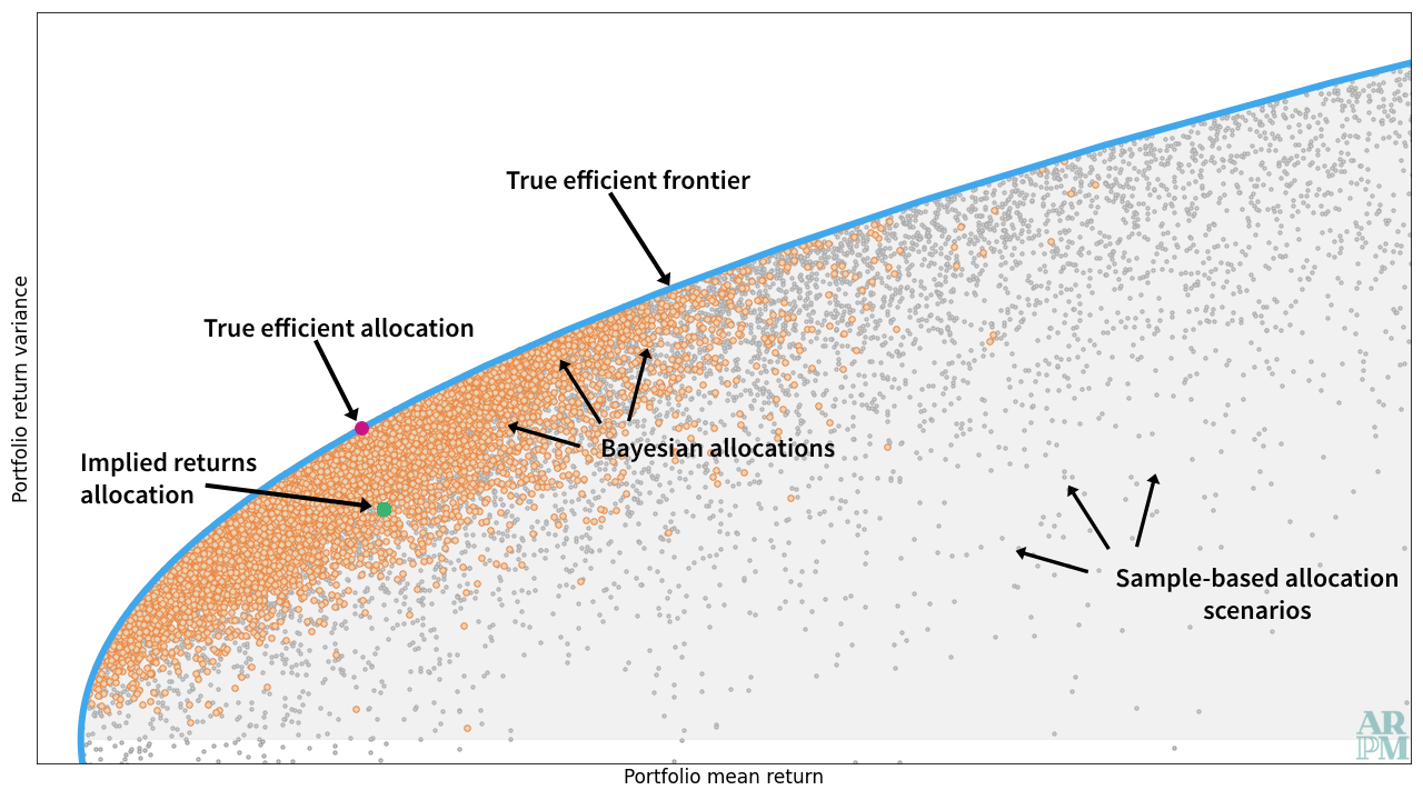
Consider the setting described in Example 60b.1, namely a market of $¯ n \equiv 3$ stocks with true mean and covariance (60b.9). We wish to estimate the efficient allocation (60b.11) for trade-off parameter $λ$ (60b.10). In this example, we consider the Bayesian allocation (60b.44). We set the prior mean and covariance as

μ^{p r i} \equiv ⎛ ⎜ ⎝ \begin{matrix} 0.47 % 0.48 % 0.30 % \end{matrix} ⎞ ⎟ ⎠, {(σ^{p r i})}^{2} \equiv ⎛ ⎜ ⎜ ⎝ \begin{matrix} {(1.52 %)}^{2} & 0 & 0 0 & {(1.53 %)}^{2} & 0 0 & 0 & {(1.20 %)}^{2} \end{matrix} ⎞ ⎟ ⎟ ⎠,

(60b.49)

so that the implied return constraint (60b.47) is enforced with the target allocation set as the equally-weighted allocation (60b.19).
We set the shrinkage parameters as

γ_{μ} \equiv 0.5, γ_{σ} \equiv 0.3,

(60b.50)

and compute the Bayesian allocations (60b.44) for each of the $¯ ȷ \equiv 1, 000$ time series of length $¯ t \equiv 22$ drawn from the true return distribution (60b.28).
Figure 60b.2 shows the mean-variance profile of the Bayesian allocations (orange), compared to the true efficient frontier (60b.4) and true efficient allocation (60b.11) (pink). We also mark sample-based allocations computed from the same samples from the true distribution (60b.28) (gray) and implied return (60b.19) (green) allocations. Notice that the Bayesian allocations display less variability than the sample-based allocations, while still using the available data.

p o r t_{B a y e s} (i) = κ \times {(γ_{σ} {(σ^{p r i})}^{2} + (1 - γ_{σ}) {ˆ σ}^{2} + γ_{μ} (1 - γ_{σ}) (μ^{p r i} - ˆ μ) {(μ^{p r i} - ˆ μ)}^{'})}_{σ}^{- 1} \times (γ_{μ} μ^{p r i} + (1 - γ_{μ}) ˆ μ - r 1),

p o r t_{ℓ o s s} (i) = p o r t_{ℓ} (i) \equiv argmin w E {ℓ (R_{¯ t + 1} - r 1, w) | i} .

M, Σ^{2} \sim f (μ, σ^{2}) .

I | μ, σ^{2} \sim f (i | μ, σ^{2}) .

R_{¯ t + 1} | i \sim f (r | i);

p o r t_{S B} (i)      sample-based large dataset ¯ t \leftarrow p o r t_{B a y e s} (i) high confidence t^{p r i}, ν^{p r i} \to p o r t_{I R} (i)      implied return .

w = q (μ, σ^{2}) \equiv \frac{λ}{2 (1 - λ)} {(σ^{2})}^{- 1} (μ - r 1) .

I | θ \sim f (i | θ) .

i \equiv {r_{t}}_{t}^{¯ t},

R_{¯ t + 1} m c \sim {μ^{*}, {(σ^{*})}^{2}},

L^{μ, σ^{2}} \equiv ℓ o s s ({μ, σ^{2}}, ˆ W) .

Θ \sim f (θ),

{I, Θ} \sim f (i, θ) = f (i | θ) \times f (θ) .

¯ ϱ (e s) \equiv E {ℓ o s s (Θ, e s (I))} = E {D (q (Θ) ∥ e s (I))} .

e s_{D} \equiv argmin e s E {D (q (Θ) ∥ e s (I))},

M_{Y, I, Θ}^{B} \equiv M_{Y, I}^{F} \cup {f (θ) : θ \in T} .

f (y | i) = \frac{f (y, i)}{\int f (˜ y, i) d ˜ y} = \int f (y | i, θ) f (θ | i) d θ,

p o r t_{ℓ o s s} (\cdot) \equiv argmin p o r t (\cdot) E {ℓ o s s ({M, Σ^{2}}, p o r t (I))}

e s_{D} = e s_{ℓ},

a^{*} \equiv a^{B a y e s} (f_{S}) \equiv argmin a \in A E {ℓ (S, a)},

ε_{t} | θ \sim f (ϵ | θ) i.i.d.

X \sim N (μ, σ^{2}),

{R_{¯ t + 1}, I, M, Σ^{2}} \sim f (r | μ, σ^{2}) f (i | μ, σ^{2}) f (μ, σ^{2});

{(Σ^{2})}^{- 1} | i \sim W i s h a r t (ν^{p o s}, \frac{1}{ν^{p o s}} {(σ^{2 p o s})}^{- 1}),

M | σ^{2}, i \sim N (μ^{p o s}, \frac{1}{t^{p o s}} σ^{2}) .

ε_{t} | (ϵ_{1}, \dots, ϵ_{¯ t}) \sim t (μ^{p o s}, \frac{t^{p o s} + 1}{t^{p o s}} σ^{2 p o s}, ν^{p o s}), t > ¯ t .

{ˆ m}_{ε}^{H i s t} \equiv {ˆ E}^{H i s t} {ε} = \frac{1}{¯ t} \sum_{t = 1}^{¯ t} ϵ_{t} .

\begin{matrix} {ˆ s}_{ε}^{2 H i s t} & \equiv {ˆ C v}^{H i s t} {ε} = \frac{1}{¯ t} \sum_{t = 1}^{¯ t} (ϵ_{t} - {ˆ m}_{ε}^{H i s t}) {(ϵ_{t} - {ˆ m}_{ε}^{H i s t})}_{t}^{'} & (24.4) = \frac{1}{¯ t} \sum_{t = 1}^{¯ t} ϵ_{t} ϵ_{t}^{'} - {ˆ m}_{ε}^{H i s t} {({ˆ m}_{ε}^{H i s t})}^{'} . \end{matrix}

γ_{μ} \equiv \frac{t^{p r i}}{t^{p r i} + ¯ t};

γ_{σ} \equiv \frac{ν^{p r i}}{ν^{p r i} + ¯ t};

p o r t_{S B} (i) \equiv \frac{λ}{2 (1 - λ)} {(\sum_{t = 1}^{¯ t} r_{t} r_{t}^{'} - \frac{1}{¯ t} (\sum_{t = 1}^{¯ t} r_{t}) {(\sum_{t = 1}^{¯ t} r_{t})}_{t}^{'})}_{t}^{- 1} \sum_{t = 1}^{¯ t} (r_{t} - r 1) .

μ_{R} = γ σ_{R}^{2} w .

p o r t_{I R} (i) \equiv {ˆ w}_{I R} .

R m c \sim {μ^{*} \equiv ⎛ ⎜ ⎝ \begin{matrix} 0.45 % 0.60 % - 0.10 % \end{matrix} ⎞ ⎟ ⎠, {(σ^{*})}^{2} \equiv ⎛ ⎜ ⎜ ⎝ \begin{matrix} {(1.50 %)}^{2} & {(0.20 %)}^{2} & {(0.09 %)}^{2} \cdot & {(1.51 %)}^{2} & {(0.50 %)}^{2} \cdot & \cdot & {(1.30 %)}^{2} \end{matrix} ⎞ ⎟ ⎟ ⎠} .

w^{*} = q (μ^{*}, {(σ^{*})}^{2}) = ⎛ ⎜ ⎝ \begin{matrix} 9.56 13.35 - 5.27 \end{matrix} ⎞ ⎟ ⎠,

λ \equiv 0.5

μ^{p r i} - {(σ^{p r i})}^{2} w^{s t r} \equiv 0,

p o r t_{I R} (i) = ⎛ ⎜ ⎝ \begin{matrix} 10.00 10.00 10.00 \end{matrix} ⎞ ⎟ ⎠,

R + 1 \sim L o g N (μ_{L o g N}, σ_{L o g N}^{2}),

w^{*} \equiv argmax w_{0} + w^{'} 1 = 1 λ E^{*} {R_{w} - r} - (1 - λ) V^{*} {R_{w} - r},

60b.2 Mean-variance Bayesian optimization

Bibliography

External Links

Discussions