


24.5 Bayesian 

Key points
- The normal-inverse-Wishart model is a tractable model for the Bayesian estimation of location and dispersion of a strong white noise.
- The estimation model is normal (24.39); the prior distribution of the parameters is normal-inverse-Wishart (24.45)-(24.46); the posterior distribution is also normal-inverse-Wishart (24.53)-(24.54), with updated parameters. The posterior predictive distribution of future instances of the strong white noise is Student t (24.62).
Bayesian estimation is discussed in full generality in Section 23.8; here we focus on the estimation of the distribution of i.i.d. variables, and in particular on one of the few analytically tractable yet non-trivial Bayesian models.
Bayesian estimation generalizes the parametric maximum likelihood approach ( Section 23.4), by modeling the unknown parameters as hidden variables.
As in classical estimation, the starting point of Bayesian estimation is an estimation model for information given hidden parameters, also known as likelihood (23.169), that is assumed true. When the data are realizations of a strong white noise (36.2), as in (23.1), such distribution is the product of the distribution of the variables
| | (24.38) |
much like the maximum likelihood approach (23.60).
In the sequel, we specialize the general exponential model (23.207) to the case of normal i.i.d. variables, which belong to the exponential family (Section 49.7.1). In this case, the conjugate prior and posterior distribution (23.210) is normal-inverse-Wishart, and the predictive distribution of the future variable , with , (23.214) is Student . We summarize the results in Table 24.8, and we proceed to discuss them.
24.5.1 Model and sample estimators
Let us assume that the i.i.d. variables are (conditionally) multivariate normal as in (24.12)
|
| (24.39) |
which is an exponential family distribution with natural parameters (49.413), sufficient statistics (49.417) and log-partition function (49.421).
From the one-to-one correspondence between natural and standard parameters (49.413), the joint likelihood (23.207) follows from (24.16) and reads 70.35
where is short notation for the historical sample mean (24.2) and is short for the historical sample covariance (24.4).
Note that, if we apply the sample mean and sample covariance estimators, (24.2) and (24.4), to a randomized time series of i.i.d. variables (23.2) distributed according to the normal model (24.39), we obtain two random variables and . More precisely, the conditional distribution of the sample mean estimator is 70.20
|
| (24.41) |
and the conditional distribution of the sample covariance estimation is 70.21
|
| (24.42) |
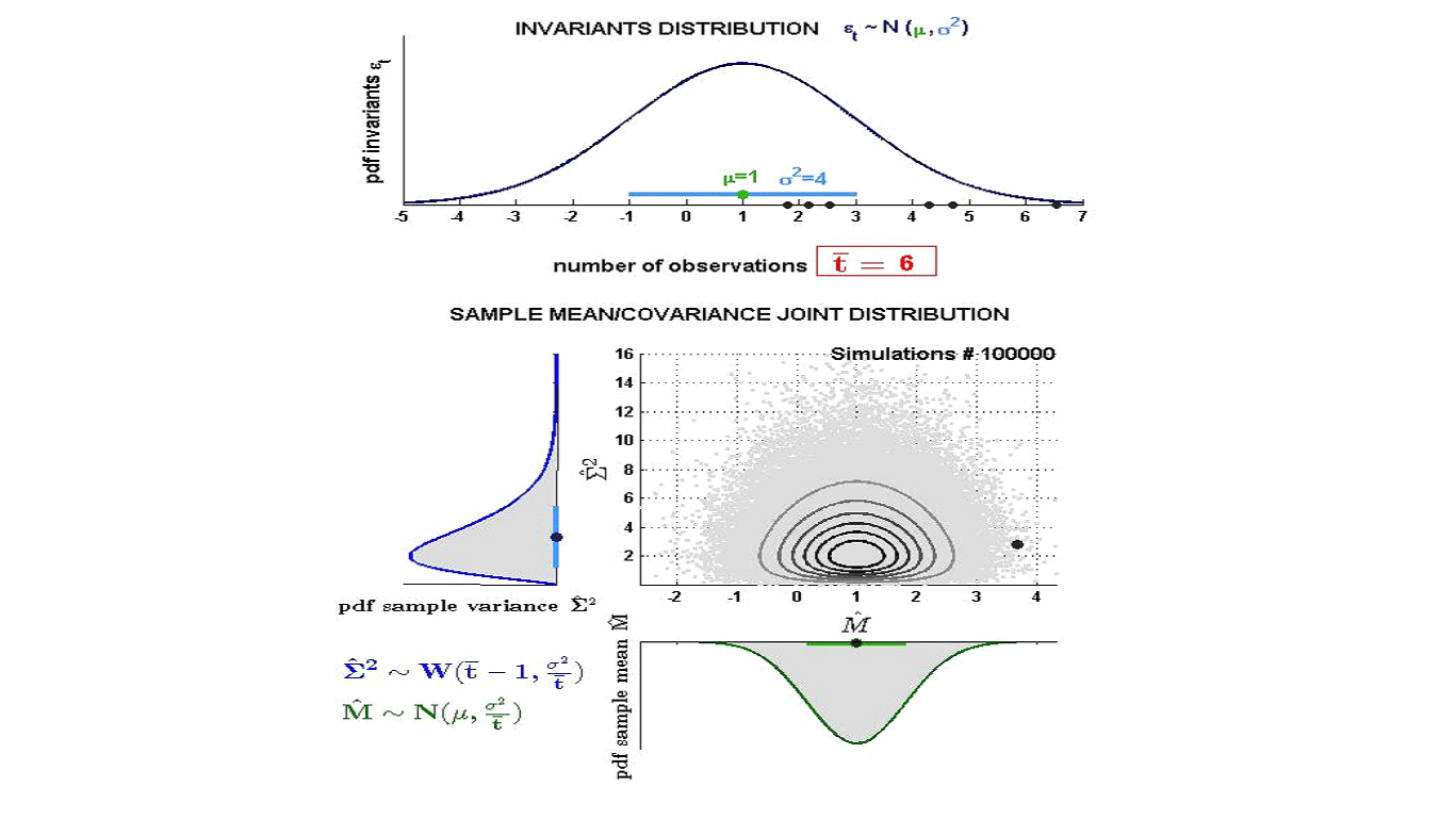
Moreover, the sample mean (24.41) and the sample covariance matrix ( 24.42) are independent random variables 70.19 . Notice that the distribution of the sample mean vector (24.41) generalizes the univariate case (27.41).
 Example 24.12. Sample mean and sample covariance distribution

Video 
Consider a normal model (24.39) in the univariate case . Figure 24.10 shows the joint and marginal distributions of sample mean (24.41) and (co)variance (24.42) as functions of the randomized time series .
24.5.2 Normal-inverse-Wishart prior distribution
Given the normal model (24.39), we assume that the natural parameters follow the conjugate distribution (23.209)
| | (24.43) |
where is given by (49.421);
|
| (24.44) |
is an symmetric and positive matrix; and is a positive scalar.
Then, the location and dispersion parameters of the conditionally normal i.i.d. variables (24.12), which are equivalent to the natural parameters , follow a normal-inverse-Wishart (NIW) distribution 70.11 . More precisely, follows an inverse-Wishart distribution (49.118)
|
| (24.45) |
and follows a multivariate normal distribution conditioning on
|
| (24.46) |
Note that the general conjugate distribution (23.209) has only one parameter to model the uncertainty of the prior. For the NIW distribution, however, we are able to specify another dispersion parameter for the location , i.e.
|
| (24.47) |
and the posterior would still be the NIW, which we will show in the next section.
The above assumptions imply that the marginal distribution of is Student , see [Murphy, 2007]
| | (24.48) |
Hence the expectation (49.137) reads
|
| (24.49) |
and the covariance (49.154) reads
|
| (24.50) |
Therefore
and
represent respectively the statistician’s prior best guess and confidence for the location
parameter.
The expectation and the covariance of the inverse-Wishart prior (24.45) read as in
(49.121)-(49.122). From the expectation of a Wishart random variable (49.109) it follows that
|
| (24.51) |
and from the covariance (49.110) we have
|
| (24.52) |
Hence we obtain that and respectively represent the statistician’s prior best guess and the confidence for the dispersion parameter.
Example 24.13. Normal-inverse-Wishart prior distribution
Video
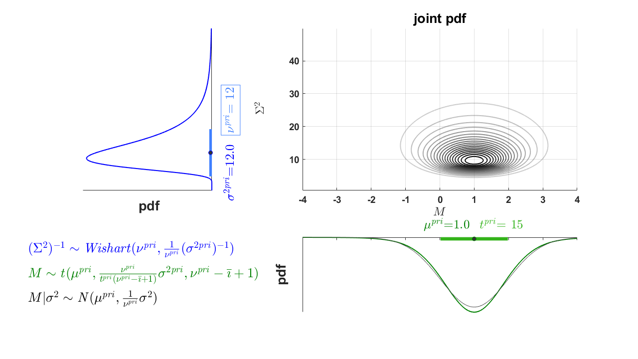
Consider a univariate i.i.d. variable, conditionally distributed as in (24.12),
with unknown location
and dispersion parameters . Then we suppose that
is univariate Wishart-distributed (24.45), or equivalently gamma (49.112), and
is
univariate normally distributed (24.47).
In Figure 24.11 we show the joint prior distribution of
by varying the
parameters .
Example 24.14. Consider the GARCH residuals (53b.36) of
stocks in the S&P 500.
We assign flexible probabilities by state-time conditioning on the VIX smoothed-scored
log-return as in Example 23.4 and we compute the corresponding HFP covariance (24.3).
Then, we shrink the HFP covariance to a correlation
(10.22) to ensure that the GARCH residuals have unit variance as in (41.76).
We want to regularize the HFP correlation
(10.22) so as to have as many null off-diagonal entries as possible
(21.86) in order to obtain a parsimonious Gaussian Markov random field structure (E.11.31).
Then, we perform Bayes estimation under the normal-inverse-Wishart model (Table 24.8)
where we set
and high confidence in the prior .
24.5.3 Normal-inverse-Wishart posterior distribution
The NIW model (24.47)-(24.45) is conjugate of the normal likelihood (24.40) and thus the posterior (23.172) is also NIW 70.12 , with parameters that can be computed analytically.
The posterior distribution of is Wishart
|
| (24.53) |
and the conditional posterior distribution of is normal
|
| (24.54) |
As a result, according to (24.48), the unconditional posterior of is Student 70.18
| | (24.55) |
In the above equations, the posterior expectation reads
|
| (24.56) |
where is the historical sample mean (24.2) and the parameter is defined using the confidence parameter for the location prior (24.47) and the sample size as
|
| (24.57) |
the posterior dispersion parameter reads
| | (24.58) |
where is the historical sample covariance (24.4) and the parameter is defined using the confidence parameter for the dispersion prior (24.45) and the sample size as
|
| (24.59) |
the parameter is
|
| (24.60) |
and is
| | (24.61) |
Refer to [Aitchison and Dunsmore, 1975] for more details.
The interpretation of the posterior parameters in (24.56)-(24.61) is the same as the prior parameters in (24.45)-(24.47), with the substitution for all the parameters.
Example 24.15. Normal-inverse-Wishart posterior distribution
Video
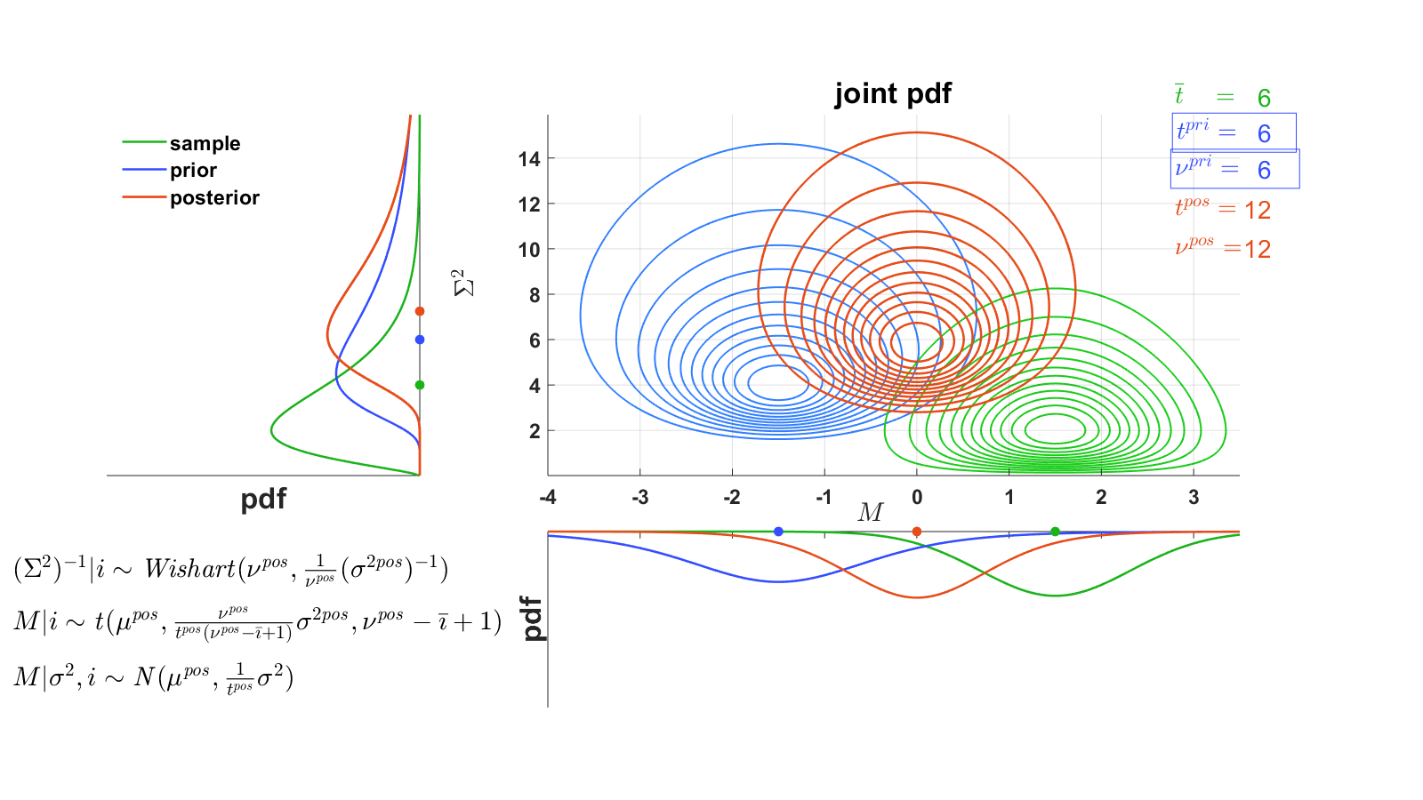
We continue from Example 24.13.
In Figure 24.12 we show three distributions:
- the joint prior distribution of
(24.45)-(24.46), with confidence parameters
- the joint distribution of sample mean and sample variance
(24.41)-(24.42), with
number of observations
- the joint posterior distribution of
(24.53)-(24.55).
As we let the confidence in the prior and the number of observations
vary,
the posterior shrinks between the prior and the sample.
For a better visualization, we assume knowledge of the true parameters to plot the sample mean
and sample variance pdf’s, keeping them fixed as the number of observations varies, similarly to
what we do in Figure 24.10 for the frequentist analysis.
Example 24.16. We continue from Example 24.14. We compute the posterior
distributions of the conditional location
(24.53) and dispersion (24.55).
24.5.4 Student t predictive distribution
From the normal model (24.12) and the normal-inverse-Wishart posterior (24.53)-(24.54), we can compute the posterior predictive distribution for the future variable (23.214), which is -distributed 70.13
| | (24.62) |
A word of reflection: the reader should not be puzzled that the i.i.d. variables , which are supposed to be independent across time (36.2), appear to be dependent under the posterior predictive distribution (24.62).
Alert 24.1. The variables are only independent conditionally given the knowledge of the
parameters ,
as shown in Example 24.17.
Example 24.17. Consider two univariate i.i.d. normal variables
| | (24.63) |
where the location parameter is a standard normal random variable
|
| (24.64) |
Then the distribution of conditional on reads 70.31
|
| (24.65) |
24.5.5 Classical equivalent, uncertainty and shrinkage
In our normal-inverse-Wishart posterior (24.53)-(24.54), the classical-equivalent (23.173) of the location parameter is , as defined in (24.56). According to the shrinkage effect (23.178), if the length of the time series is large, then the parameter shrinks towards the sample mean ; instead, it shrinks towards the prior when it is the confidence in the prior to be large
|
| (24.66) |
On the other hand, one possible classical-equivalent of the dispersion parameter is as defined in (24.58), which satisfies . Similar to the location, the parameter shrinks towards the sample covariance if the length of the time series is large; instead, it shrinks towards the prior when the confidence in the prior is large
| | (24.67) |
The classical-equivalent has a slightly more complex expression when defined as the mode (23.174) of the posterior distribution 70.16 -70.14 .
When , we recover the general shrinkage (23.213) for exponential family
|
| (24.68) |
 Example 24.18. In Figure 24.12 we highlight the shrinkage effects (24.66) and
(24.67) of the classical equivalent.
Example 24.18. In Figure 24.12 we highlight the shrinkage effects (24.66) and
(24.67) of the classical equivalent.
Example 24.19. Bayesian estimation: stocks
We continue from Example 24.16. Our regularized estimate for the location
and dispersion are the classical-equivalent parameters (23.173), respectively
(24.56)
and
(24.58).
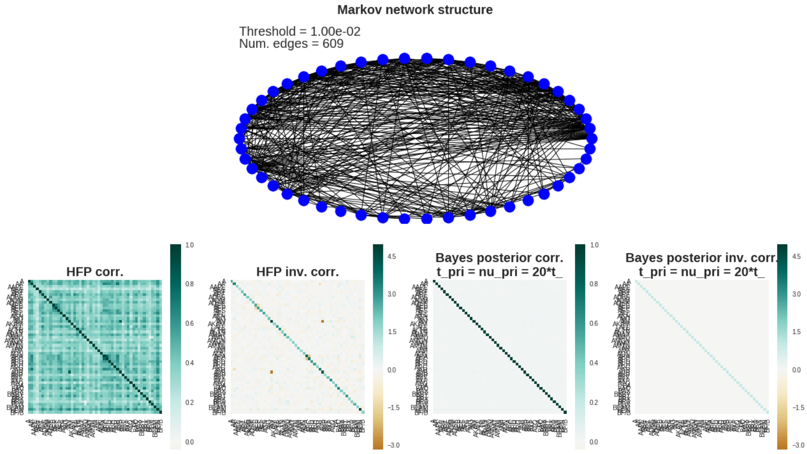
In the bottom plots Figure 24.13 we show:
-) the HFP correlation (24.3)-(10.22)
and the corresponding inverse correlation
(left);
-) the Bayes posterior (24.58)
and the corresponding inverse
(right).
We observe that as the confidence in the prior
increases, the off-diagonal
terms in the Bayes posterior
converge to
as follows from the shrinkage effect (24.67).
In the top plot of Figure 24.13, we show the Gaussian Markov random field (21.85) structure of the i.i.d.
variables (see Section 24.6.5), where the edges are missing if the absolute value of the corresponding
entry of the inverse covariance falls below a given threshold (21.86). The more the confidence in the
prior
increases, the more parsimonious the conditional independence (E.11.31) structure. Refer to
Example 24.27 to compare with the glasso regularization.
The posterior of the expectation is -distributed (24.55) like the prior (24.48) and hence the uncertainty in the estimate of the expectation, as defined in (23.175), reads
|
| (24.69) |
It is immediate to verify that the uncertainty (24.69) shrinks to zero in the presence of a long time series or high confidence in the prior, according to the shrinkage effect (23.180).
On the other hand, the posterior of the covariance follows an inverse-Wishart distribution (24.53) like the prior (24.45) and then the uncertainty of the covariance estimate, as defined in (23.175), reads similarly to (24.52)
|
| (24.70) |
where is the commutation matrix (43.592). If we choose the modal square-dispersion (23.176) as uncertainty for the posterior distribution of we obtain different expressions 70.17 -70.15 . Again, it is immediate to verify that the uncertainty (24.70) and its alternative formulations shrink to zero in the presence of a long time series or high confidence in the prior, according to the shrinkage effect (23.180).
Example 24.20. In Figure 24.12 we highlight the shrinkage effect (23.180) for the
uncertainty of location
(24.69) and of dispersion
(24.70).